Mixing quantum computing and Artificial Intelligence (AI) may sound like a new buzzword. However, since quantum computing advances are hinting at profound changes in the very notions of computation, it is natural to reexamine various branches of computer science in the light of these disruptions. And … AI is no exception
As usual, before entering the quantum realm, it is important to get an overview of the classical world.
AI, Machine Learning, Artificial Neural Networks & Deep Learning
Artificial Intelligence is difficult to define. Probably because intelligence, by itself, is difficult to define. AI is often defined as the study of any device that perceives its environment and takes actions that maximize its chance of successfully achieving its goals. In day to day situations, the term AI applies when a machine perform tasks that normally require human intelligence, such as learning, reasoning, problem solving, decision-making, planning, visual perception, knowledge representation, natural language processing, competing at the highest level in strategic game systems or driving cars.
The AI field draws upon computer science, mathematics, psychology, linguistics and many others. Approaches to AI include include statistical methods, computational intelligence, or traditional symbolic AI. To reach its goals, many tools are used in AI, including search and mathematical optimization, artificial neural networks, and methods based on statistics, probability and economics.
Along its history, AI has seen many ups and downs. As of 2018, AI techniques have experienced a resurgence following concurrent advances in computer power, large amounts of data, and theoretical understanding. Nowadays, AI techniques have become an essential part of the industry.
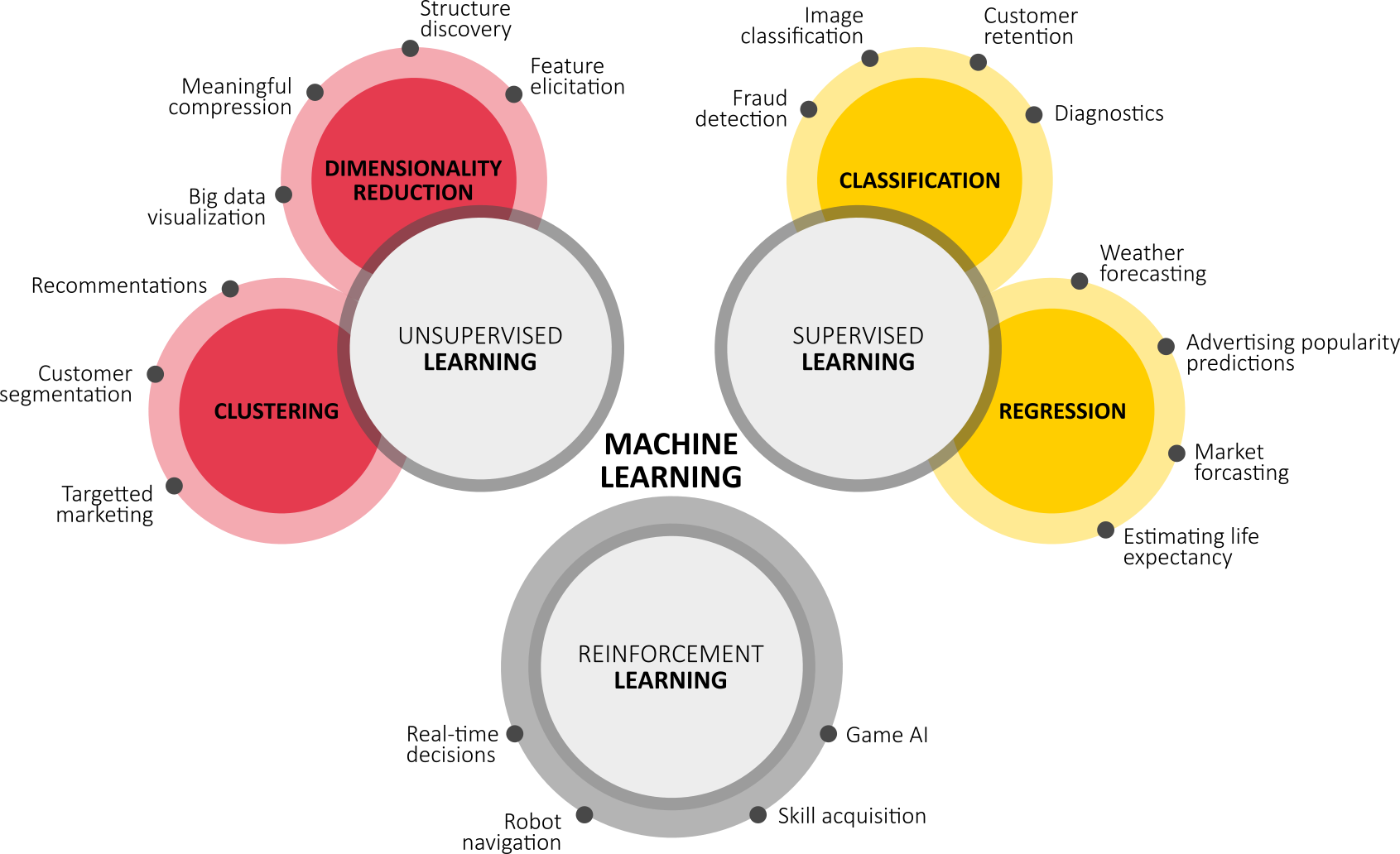
Machine learning (ML) was first defined by Arthur Samuel in 1959. It is a subset of artificial intelligence that uses statistical techniques to give computers the ability to learn (i.e., progressively improve performance on a specific task) with data, without being explicitly programmed. Machine learning algorithms operate by constructing a model with parameters that can be learned from a large amount of example inputs, called a training set.
Machine learning is typically classified into three broad categories (leading to different typical applications):
- Supervised learning: the computer is presented with example inputs and their desired outputs, given by a “teacher”, and the goal is to learn a general rule that maps inputs to outputs. As special cases, the input signal can be only partially available, or restricted to special feedback:
- Unsupervised learning: no labels are given to the learning algorithm, leaving it on its own to find structure in its input. Unsupervised learning can be a goal in itself (discovering hidden patterns in data) or a means towards an end (feature learning);
- Reinforcement learning: inspired by behaviourist psychology, reinforcement learning is concerned with how software agents ought to take actions in an environment so as to maximize some notion of cumulative reward.
There are so many approaches to Machine Learning that it is difficult to get an exhaustive overview of ML algorithms. This selected list tries to summarize the most common approaches :
- Decision tree learning uses a decision tree as a predictive model, which maps observations about an item to conclusions about the item’s target value;
- Support vector machines (SVM) are a set of related supervised learning methods used for classification and regression. Given a set of training examples, each marked as belonging to one of two categories, an SVM training algorithm builds a model that predicts whether a new example falls into one category or the other;
- Genetic algorithm (GA) is a search heuristic that mimics the process of natural selection, and uses methods such as mutation and crossover to generate new genotype in the hope of finding good solutions to a given problem;
- Cluster analysis is the assignment of a set of observations into subsets (clusters) so that observations within the same cluster are similar according to some predesignated criterion or criteria, while observations drawn from different clusters are dissimilar;
- Bayesian networks (or belief networks) are probabilistic graphical models that represents a set of random variables and their conditional independencies via directed acyclic graphs. They are used for inference and learning;
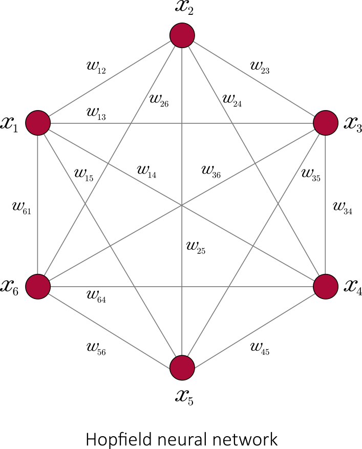
- Artificial neural network are learning algorithm inspired by biological neural networks. Computations are structured in terms of an interconnected group of artificial neurons, processing information. Modern neural networks are non-linear statistical data modeling tools. They are usually used to model complex relationships between inputs and outputs, to find patterns in data, or to capture the statistical structure in an unknown joint probability distribution between observed variables.
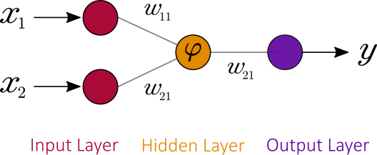
Let us focus on Artificial Neural Networks. The first formal artificial neuron model was proposed by Warren McCulloch and Walter Pitts in 1943.
For a given artificial neuron 


In the McCulloch-Pitts model, a Heaviside step function was used as a transfer function. Nowadays, a sigmoid function ![\varphi(x) \in ]-1,+1[](https://s0.wp.com/latex.php?latex=%5Cvarphi%28x%29+%5Cin+%5D-1%2C%2B1%5B&bg=ffffff&fg=000000&s=0 "\varphi(x) \in ]-1,+1[")
![]()
To combine these neurons together, one uses the output of a neuron as one the inputs of another neuron. Combined together, neurons can act as any logical gate. Furthermore, if one introduces loops in the neural network, it can be used as a Turing machine.
In the case where 

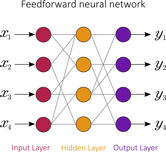
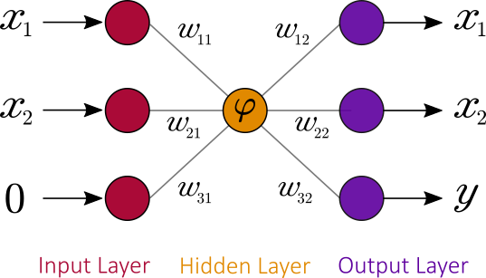
Conversely, a feedforward neural network is an artificial neural network wherein connections between the nodes do not form a cycle:
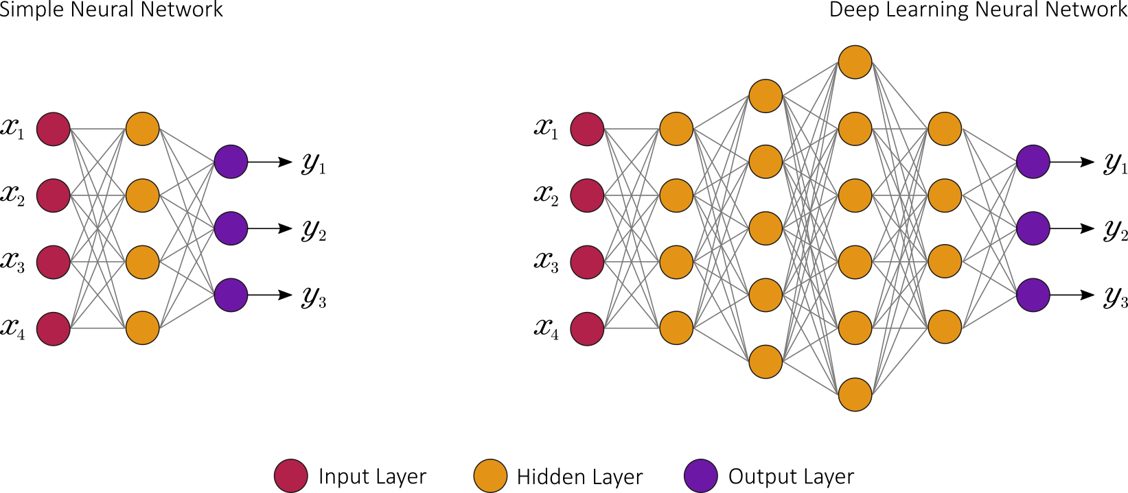
Deep learning (DL) is a subset of machine learning. It utilizes a hierarchical level of artificial neural networks to carry out the process of machine learning. While traditional programs build analysis with data in a linear way, the hierarchical function of deep learning systems enables machines to process data with a nonlinear approach.
DL is a specific approach used for building and training neural networks. An algorithm is considered to be deep if the input data is passed through a series of nonlinear transformations before it becomes output.
DL removes the manual identification of features in data and, instead, relies on whatever training process it has in order to discover the useful patterns in the input examples. This makes training the neural network easier and faster, and it can yield a better result.
Be it classical or quantum, the main job of artificial neural networks is to recognize patterns. Do to so, when data is fed into the network, each artificial neuron that fires transmits a signal to certain neurons in the next layer, which are likely to fire if multiple signals are received.
The first layer of the neural network processes a raw data input and passes it on to the next layer as output. A second layer processes the previous layer’s information by including additional information and passes on its result. The next layer takes the second layer’s information and, in turn, includes other raw data to make the machine’s pattern even better. This continues across all levels of the neuron network:
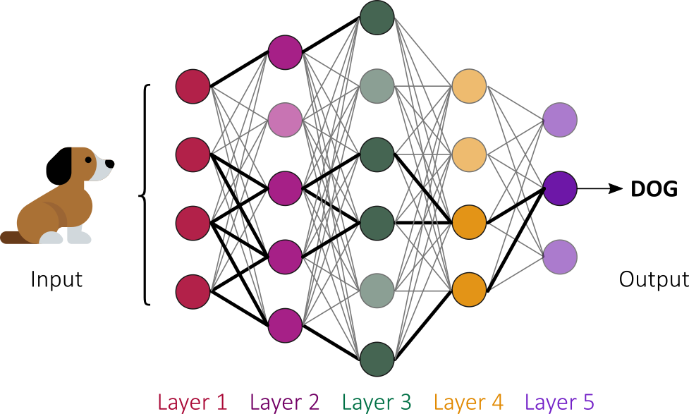
The process filters out noise and retains only the most relevant features. The initial layer accepts input (such as the pixels of an image), intermediate layers create various combinations of the input (representing structures such as edges and geometric shapes) and a final layer produces output (a high-level description of the image content). The “wiring” is not fixed in advance, but adapts in a process of trials and errors.
On a classical computer, all these interconnections are represented by an enormous matrix of numbers. Running the network means doing matrix algebra. Typically, these heavy matrix operations are outsourced to specialized chips such as a GPUs (Graphics Processing Units).
And this is where quantum computing can enters.
Amplitude encoding
Let’s explore the impact of quantum computing on AI with amplitude encoding.
Generally speaking, two qubits system have four joint states:
;
;
;
.
Let’s associate the probability amplitudes of a quantum state with the inputs and outputs of computations. Each state has a certain amplitude (or weight) that can represent a neuron.
If you add a third qubit, you can represent eight neurons; a fourth, 16. Since a state of n qubits is described by complex amplitudes, this information encoding can allow for an exponentially compact representation.

It is estimated that 60 qubits would be enough to encode an amount of data equivalent to that produced by humanity in a year.
When you act on a state of four qubits, you are processing 16 numbers at a stroke, whereas a classical computer would have to go through those numbers one by one. The goal of algorithms based on amplitude encoding is to formulate quantum algorithms whose resources grow polynomially in the number of qubits, which amounts to a logarithmic growth in the number of amplitudes and thereby the dimension of the input.
Quantum algorithm for linear systems (HHL)
Nevertheless, quantum computers’ ability to store information compactly doesn’t make it faster. In 2009, Seth Lloyd and Aram Harrow from the MIT and Avinatan Hassidim from the Bar-Ilan University in Israel, designed a crucial quantum algorithm (now known as the HHL algorithm) to for solving linear systems 
Exploring the details of HHL goes beyond this post, but you can have a look at their seminal paper “Quantum algorithm for solving linear systems of equations“.
To be precise, HHL is not exactly an algorithm for solving a system of linear equations in logarithmic time. Rather, it’s an algorithm for preparing a quantum superposition of the form 

Even though HHL has known caveats, it is one of the most important subroutines in many quantum machine learning algorithms.
For example, the quantum algorithm for linear systems of equations has been applied to a support vector machine. Rebentrost et al. have shown that a quantum support vector machine can be used for big data classification and achieve an exponential speedup over classical computers.
Amplitude amplification
The HHL algorithm is one of the main fundamental algorithms expected to provide a speedup over their classical counterparts, along with Grover’s search algorithm or Shor’s factoring algorithm:

Another approach to improving classical machine learning with quantum information processing uses amplitude amplification methods based on Grover’s search algorithm:

Many AI problems can be reduced to searching: planning, scheduling, theorem proving, etc. Indeed, it has been shown that amplitude amplification can solve unstructured search problems with a quadratic speedup compared to classical algorithms.
These quantum routines can be employed for learning algorithms that translate into an unstructured search task, as can be done for instance in the case of the k-medians and the k-nearest neighbors algorithms. Amplitude amplification is often combined with quantum walks to achieve the same quadratic speedup. Quantum walks have been proposed to enhance Google’s PageRank algorithm for example.
Quantum Neural Networks
Computer scientists are trying to combine artificial neural network models with the advantages of quantum information in order to develop more efficient algorithms. The hope is that features of quantum computing such as quantum parallelism or the effects of interference and entanglement can be used as resources. One important motivation for these investigations is the difficulty to train classical neural networks, especially in big data applications.
Quantum neural network research is still in its infancy. Most of the proposed models are based on the idea of replacing classical McCulloch-Pitts neurons with a qubit (sometimes called a “quron”), resulting in neural units that can be in a superposition of the state ‘firing’ and ‘resting’:
- The McCulloch-Pitts neuron
is replaced by a qubit (quron)
in 2-dimensional Hilbert space
with basis
;
- The state
of a network of
qurons becomes then a quantum state in a
-dimensional Hilbert space
with basis
.
- The initial state of the quantum system encodes any binary string of length.
- The QNN reflects one or more basic neural computing mechanisms (attractor dynamics, synaptic connections, integrate & fire, training rules, …)
- The evolution is based on quantum effects, such as superposition, entanglement and interference, and it is fully consistent with quantum theory.
Let’s have a look on how QNN could be applied to feedforward neural network:
Two problems arise with regard to quantum computations:
- The quantum operations need to be reversible and unitary. The classical transfer function
is not reversible as it squeezes the two dimensional vector to a single number
;
- Due to the no-cloning theorem, the copying of the output before sending it to several neurons in the next layer is non-trivial
In order to fix irreversibility of classical neural networks, a dummy bit in state 

The last step is to change reversible function 
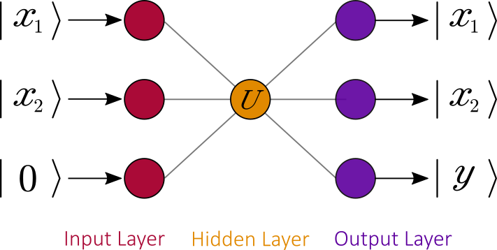
qubits can be represented as :![\displaystyle U = \textrm{exp}\Big[ i \big( \sum_{k_1,\cdots, k_n} \alpha_{k_1,\cdots, k_n} (\sigma_{k_1}\otimes\cdots\otimes\sigma_{k_n})\big)\Big]](https://s0.wp.com/latex.php?latex=%5Cdisplaystyle+U+%3D+%5Ctextrm%7Bexp%7D%5CBig%5B+i+%5Cbig%28+%5Csum_%7Bk_1%2C%5Ccdots%2C+k_n%7D+%5Calpha_%7Bk_1%2C%5Ccdots%2C+k_n%7D+%28%5Csigma_%7Bk_1%7D%5Cotimes%5Ccdots%5Cotimes%5Csigma_%7Bk_n%7D%29%5Cbig%29%5CBig%5D+&bg=ffffff&fg=000000&s=0 "\displaystyle U = \textrm{exp}\Big[ i \big( \sum_{k_1,\cdots, k_n} \alpha_{k_1,\cdots, k_n} (\sigma_{k_1}\otimes\cdots\otimes\sigma_{k_n})\big)\Big]")
where 


This is a different approach in comparison to classical neural networks as the transfer functions (instead of numeric weights) represented by unitary matrices are trainable.
The benefits of quantum neural networks in comparison to the classical algorithm are not yet specified. A potential speed-up can come from a superposition, however the assessment of unitary matrix learning speed is difficult. Nevertheless, the quantum neural networks algorithm is an interesting and promising field of quantum machine learning algorithms that is currently under development.
Quantum Boltzmann Machine
A Boltzmann machine (BM) is a type of stochastic recurrent neural network (and Markov random field). They are named after the Boltzmann distribution in statistical mechanics (this is why they are classified as Energy Based Models). BMs are classic machine learning techniques, and serve as the basis of deep learning models such as deep belief networks and deep Boltzmann machines.
A BM commonly consists of visible and hidden binary units 
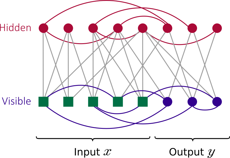
The quadratic energy function over binary units

where the dimensionless parameters 


The goal is to determine the Hamiltonian parameters 


To jump into the quantum realm, we now replace classical bits with qubit:
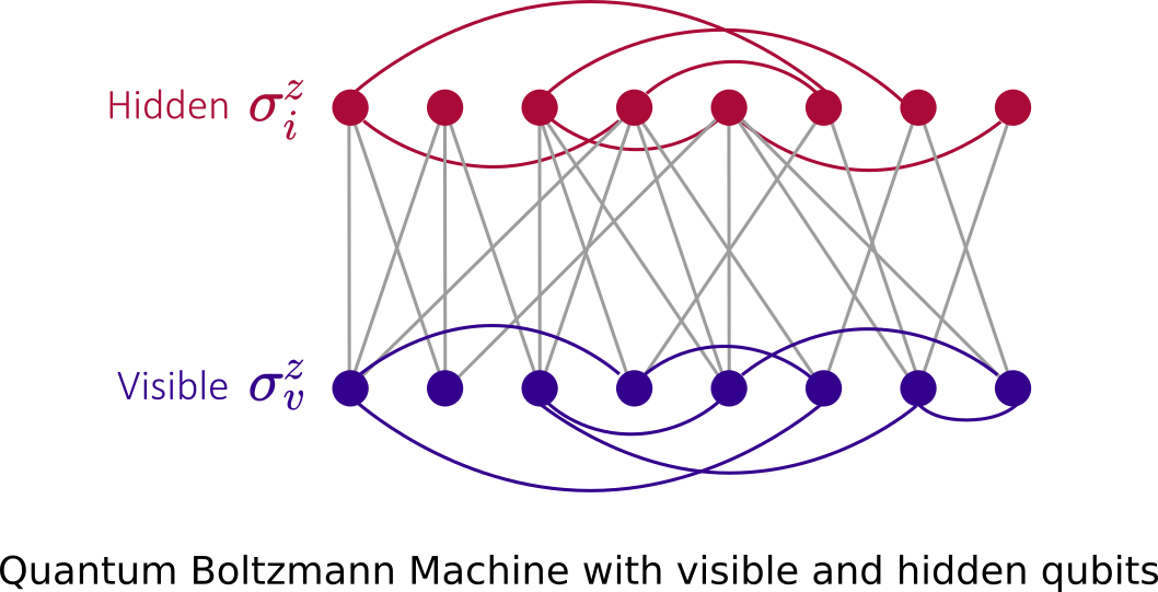
For the energy function, one will then considers the Hamiltonian:
with
and the Pauli matrix


The standard approach to training Boltzmann machines relies on the computation of certain averages that can be estimated by standard sampling techniques, such as Markov chain Monte Carlo algorithms. Another possibility is to rely on a physical process, like quantum annealing, that naturally generates samples from a Boltzmann distribution.
The objective is to find the optimal control parameters that best represent the empirical distribution of a given dataset.
Other approaches
There many other approaches to quantum AI, and a simple post won’t be nearly enough to get into all of them. To name a few:
- Quantum principal component analysis
- Quantum k-means algorithm
- Quantum k-medians algorithm
- Quantum Bayesian Networks
- etc.
I would recommend this paper to explore a few of them in an accessible and consistent way: Quantum machine learning for data scientists.
Note: A few paragraphs and illustrations of this post are based selected papers on quantum AI and wikipedia articles.