In a series of posts, we introduced various quantum computing concepts:
- How information and quantum mechanics are related ?
- What is quantum computing ?
- What are Bell states ?
- What is quantum teleportation ?
- What is quantum error correction ?
- What are topological quantum computer ?
In addition to these concepts, we devoted two posts to the very crucial topic that is complexity:
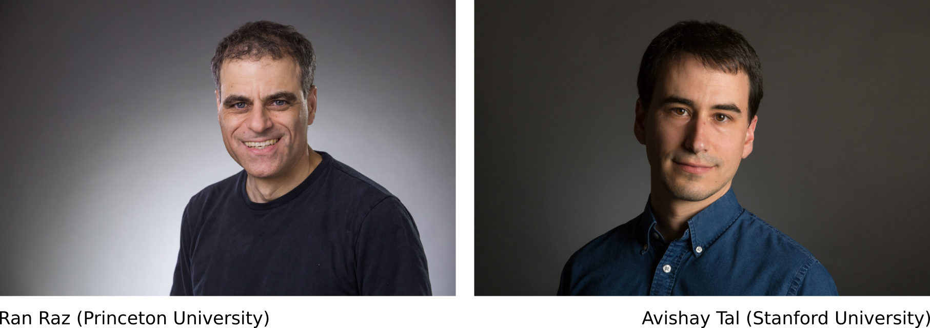
In a recent paper, computer scientists Ran Raz and Avishay Tal rocked the world of quantum complexity so much it is now time for an update on that subject !
Back to complexity classes
One of the purposes of theoretical computer science is to sort problems into complexity classes. Quoting Quanta Magazine, a complexity class “contains all problems that can be solved within a given resource budget, where the resource is something like time or memory.”
In a previous post, we have introduced the two most famous complexity classes:
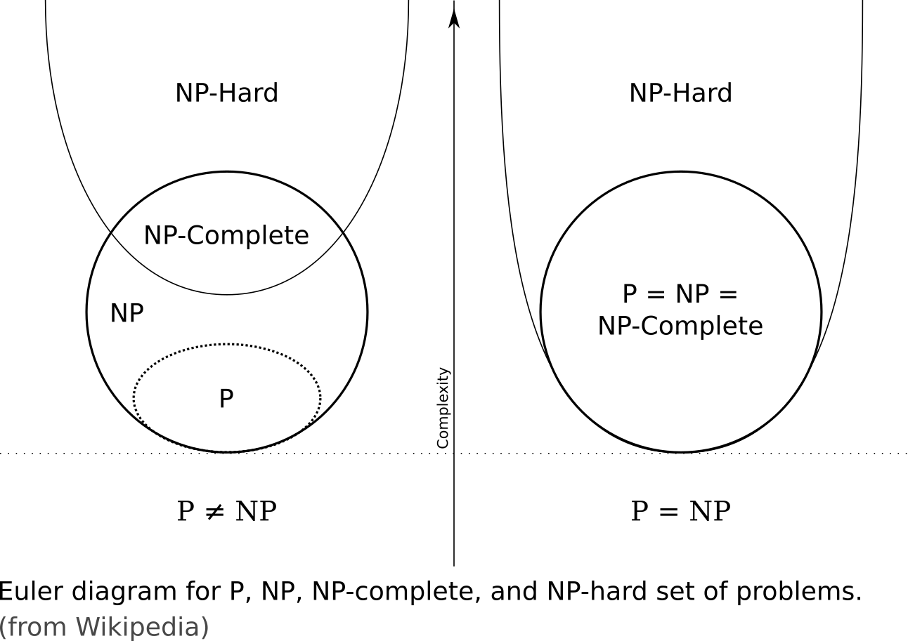
- P: The complexity class of decision problems that can be solved on a deterministic Turing machine in polynomial time. P is all the problems that a classical computer can solve quickly (for example: “Is this number prime?” belongs to P).
- NP: The complexity class of decision problems that can be solved on a non-deterministic Turing machine in polynomial time. NP is all the problems that classical computers can’t necessarily solve quickly, but for which they can quickly verify an answer if presented with one. (for example: “What are its prime factors?” belongs to NP).
Also, within the NP class, we introduced NP-complete and NP-hard problem (a problem is said to be NP-hard if an algorithm for solving it can be translated into one for solving any NP-problem), as well as NP-intermediate (NPI) class (problems in the complexity class NP but that are neither P nor NP-complete).
co-NP is the complexity class which contains the complements of problems found in NP. In other terms, class of problems for which there is a polynomial-time algorithm that can verify counterexamples.
Determining whether it is possible to solve these problems quickly, called the P versus NP problem, is one of the principal unsolved problems in computer science today:
Quantum complexity
In 1993 computer scientists Ethan Bernstein and Umesh Vazirani defined a new complexity class called BQP (for Bounded-error Quantum Polynomial time): the complexity class of decision problems that can be solved with 2-sided error on a quantum Turing machine in polynomial time.
They defined this particular class to contain all the decision problems that quantum computers can solve efficiently. They also proved that quantum computers can solve all the problems that classical computers can solve : BQP contains all the problems that are in P.
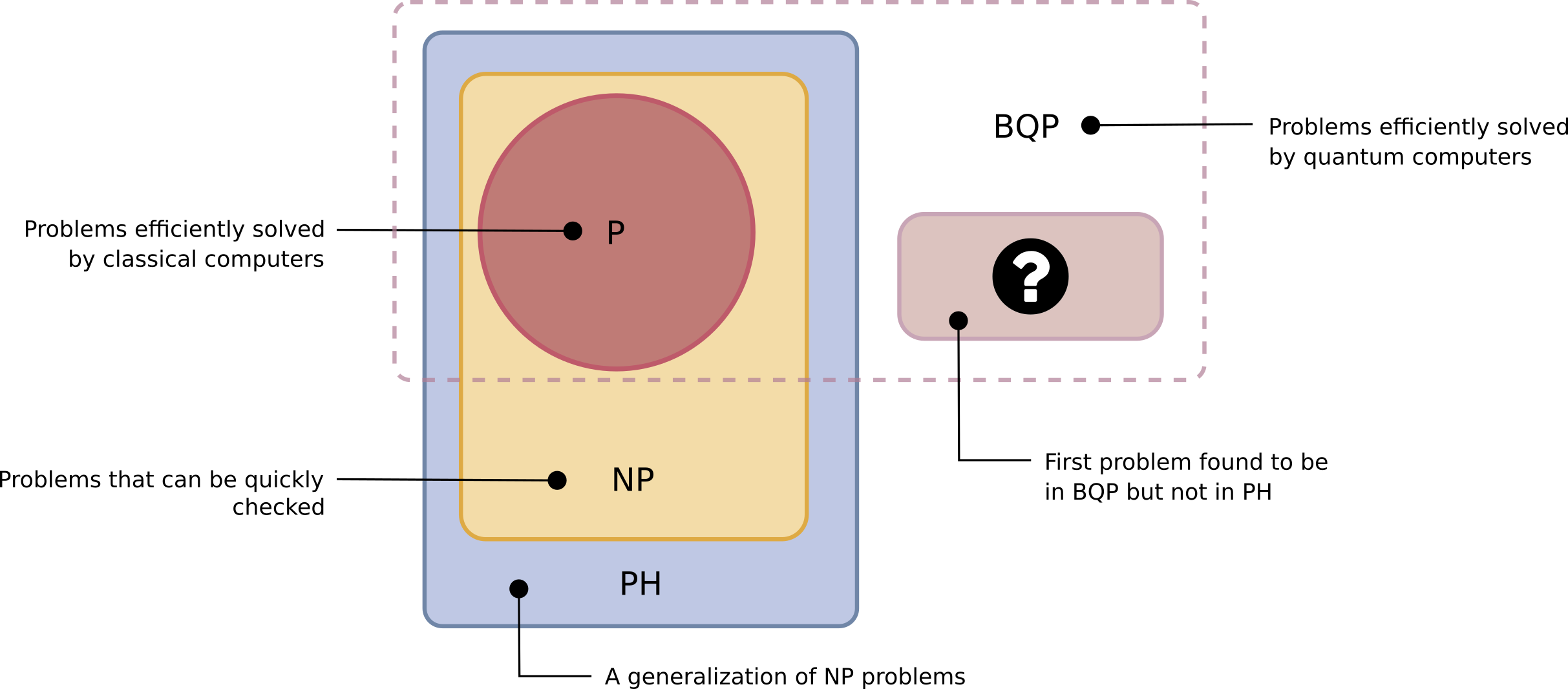
A central task of quantum computing theory is to understand how BQP fits in with classical complexity classes. That is why the boundaries of BQP, sketched in the following diagram, are uncertain:
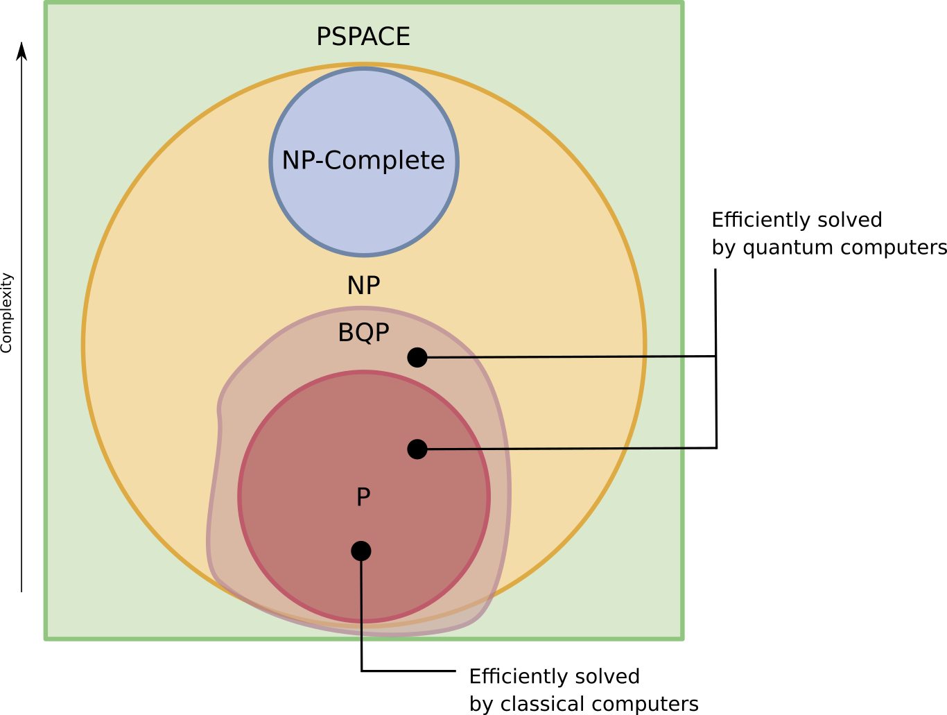
So far, we know that:
- P sits in BQP
- BQP sits in PSPACE
- Boundaries of BQP (relative to NP) are uncertain
The complexity class PH is the union of all complexity classes in the Polynomial Hierarchy. PH is the is a generalization of NP to allow multiple quantifiers such as ∃ (i.e. there exists), ∀ (i.e. for all), etc. (see second order logic for details).
You can think of PH as the class of all problems classical computers could solve if P turned out to equal NP.
In other words, to compare BQP and PH is to “determine whether quantum computers have an advantage over classical computers that would survive even if classical computers could solve many more problems than they can today“ [Quanta Magazine].
Using oracle separation to distinguish BQP from PH
Up to now, there were some evidence that BQP was not contained in PH. This result is now proven by Ran Raz and Avishay Tal.
The best way to distinguish between two complexity classes is to find a problem that is provably in one and not the other.
If you want a problem that is in BQP but not in PH, you have to identify something that “by definition a classical computer could not even efficiently verify the answer, let alone find it,” (Scott Aaronson).
The first step was the introduction of the concept of “forrelation” (also known as Fourier checking) by Scott Aaronson and Andris Ambainis. See for example:
The problem to be solved is the following:
- Imagine two random number generators (f and g), each producing a sequence of bits
- Forrelation estimates the correlation between f and the Fourier transform of g (are the two sequences completely independent from each other, or are they related in a hidden way)
It was then proved in 2010 that forrelation belongs to BQP. What is left was the hardest step: proving that forrelation is not in PH.
To distinguish between complexity classes like BQP and PH, one would like be to measure the computational time required to solve a problem in each. Unfortunately, nobody has a clear understanding of how to measure actual computation time.
When the thing they’d really like to prove is beyond their reach, computer scientists often resort to oracles. They measure something else that they hope will provide insight into the computation times they can’t measure: they work out the number of times a computer needs to consult an oracl” in order to come back with an answer.
We can get an understanding of complexity by allowing both machines access to the same oracle and seeing what we can separate. In our case, the problem is to figure out whether two random number generators are secretly related:
- You can ask the oracle questions such as “What’s the sixth number from each generator?”.
- Then you compare computational power based on the number of hints each type of computer needs to solve the problem. The computer that needs more hints is slower.
The paper published by Ran Raz and Avishay Tal shows that quantum computer need just one hint, while even with unlimited hints, there’s no algorithm in PH that can solve the problem.
“This means there is a very efficient quantum algorithm that solves that problem,” said Raz. “But if you only consider classical algorithms, even if you go to very high classes of classical algorithms, they cannot.”
Quantum and classical computers exist in a different computational realm
This establishes that with an oracle, Fourier checking (forrelation) is a problem that is in BQP but not in PH. This is big, so let’s repeat it : for the first time, a problem is found to be in BQP but not in PH:
To finish this update, let’s quote Quanta Magazine: “The work provides an ironclad assurance that quantum computers exist in a different computational realm than classical computers (at least relative to an oracle). Even in a world where P equals NP […] Raz and Tal’s proof demonstrates that there would still be problems only quantum computers could solve. Even if P were equal to NP, even making that strong assumption,” said Fortnow, “that’s not going to be enough to capture quantum computing.”
Note: A few paragraphs and illustrations of this post are based on Quanta Magazine.