On photonic quantum computing

The worldwide quest to build practical quantum computers is undergoing a critical period. Fault-tolerant quantum computers will soon provide significant computational speedups for problems like factoring, search, or linear algebra, etc. During the next few years, a number of different quantum devices will become available to the public.

Over the past decade, a wide variety of physical architectures have been investigated for their suitability for quantum technologies, including (among others) trapped atoms and ions quantum computers, topological quantum computers, or photonic quantum computers.

In 2000 by E. Knill, R. Laflamme and G. Milburn proposed a protocol (now named KLM scheme) using photons as information carriers to implement linear optical quantum computing. This protocol makes it possible to create universal quantum computers solely with linear optical tools.

Photons

Let’s start first with a general recap on photons, which are elementary spin-1 particles. By virtue of their integer spin, they are bosons (as opposed to fermions with half-integer spin). By the spin-statistics theorem, all bosons obey Bose–Einstein statistics (whereas all fermions obey Fermi–Dirac statistics). As such, they do not obey the Pauli exclusion principle restrictions (no two identical fermions may occupy the same quantum state simultaneously).

The following image sketches the difference between bosons and fermions:

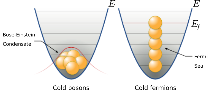
Imagine two apparati, one containing a gas of bosons, while the other one contains a gas of (non interacting) fermions. As the temperature drops near absolute zero, the gas of bosons collapses, forming a Bose-Einstein Condensate. Fermions can’t reach this state, since they can’t occupy the same quantum state. The total energy of the Fermi gas is then larger than the sum of the single-particle ground state. The energy of the highest occupied quantum state is called the Fermi energy.

At the most elementary level, one can see fermions as the perfect candidate for building blocks of matter, while bosons are candidates for interactions. As such, photons are the carriers of the electromagnetic interaction.

Photons are indeed the quantum of the electromagnetic field which is understood as a gauge field, i.e., as a field that results from requiring that a gauge symmetry holds independently at every position in spacetime. For the electromagnetic field, this gauge symmetry is the Abelian U(1) symmetry, which reflects the ability to vary the phase of a complex field without affecting observables such as the energy or the Lagrangian.

The quanta of an Abelian gauge field must be massless, uncharged bosons, as long as the symmetry is not broken. The photon thus is massless, moves at the speed of light in vacuum, has zero electric charge.

Each photon carries one quantum of energy, equal to $\hbar\omega$ (where $\omega$ is its angular frequency). Photons are emitted in many natural processes. For example:

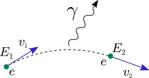
When a charge is accelerated it emits synchrotron radiation:

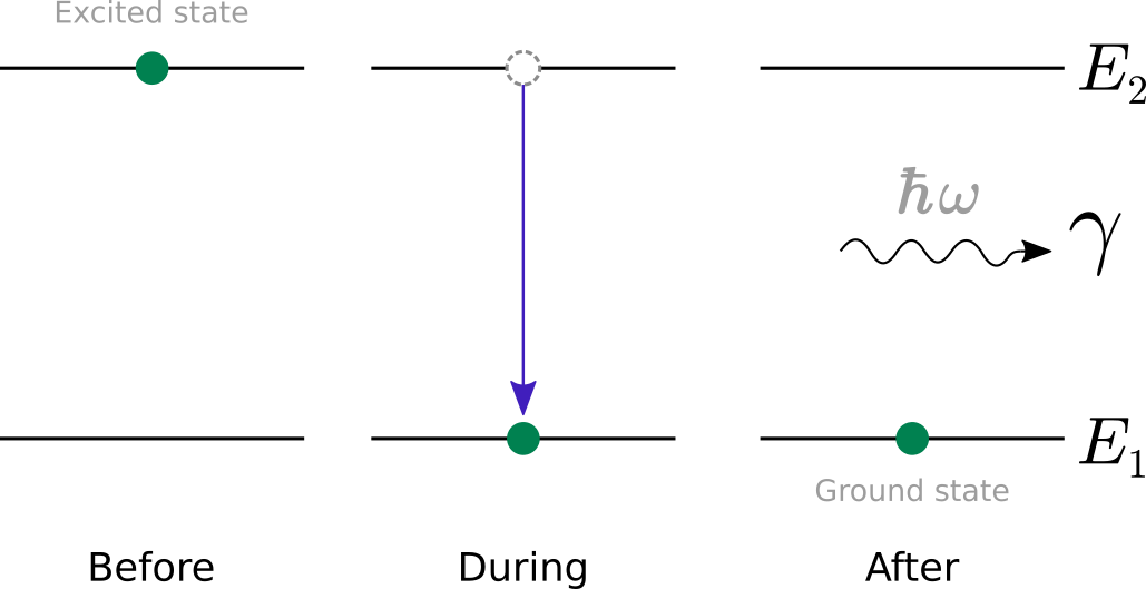
During an atomic or nuclear transition to a lower energy level, photons of various energy will be emitted, ranging from radio waves to gamma rays. The energy possessed by a single photon corresponds exactly to the transition between the discrete energy levels that emitted the photon:

Photons can also be emitted when a particle and its corresponding antiparticle are annihilated, like in the following annihilation diagrams:

Quantum computing with linear quantum optics has the advantage that its smallest unit of quantum information (the photon) is potentially free from decoherence: the quantum information stored in a photon tends to stay there.

The downside is that photons do not naturally interact with each other, and in order to apply 2-qubit quantum gates such interactions are essential.

Linear Optical Quantum Computing

There are many implementations for quantum information processing and quantum computation. Optical quantum systems are interesting candidates because they link quantum computation and quantum communication within a same framework.

Linear Optical Quantum Computing (LOQC) uses (mostly) linear optical elements to process quantum information, photon detectors and quantum memories to detect and store quantum information. These optical elements uses combinations of beam splitters, phase shifters, and mirrors:

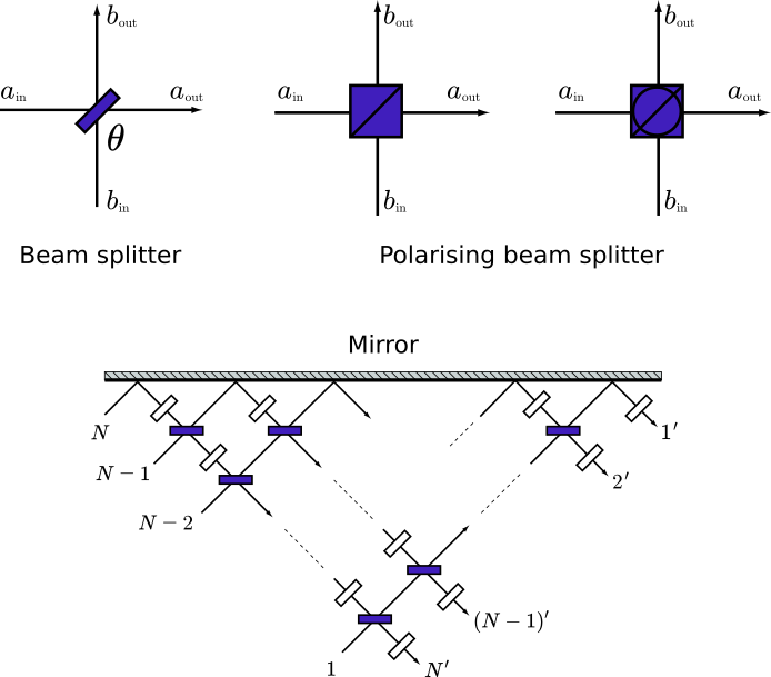
Each linear optical element equivalently applies a unitary transformation on a finite number of qubits. This network of finite linear optics can realize any quantum circuit.

Operations via linear optical elements preserve the photon statistics of input light. For example

a coherent (classical) light input produces a coherent light output
a superposition of quantum states input yields a quantum light state output.

An intrinsic problem in using photons as information carriers is that photons hardly interact with each other. This potentially causes a scalability problem for LOQC, since nonlinear operations are hard to implement, which can increase the complexity of operators and hence can increase the resources required to realize a given computational function.

One way to solve this problem is to bring nonlinear devices into the quantum network. For instance, the Kerr effect can be applied into LOQC to make a single-photon CNOT gate and other operations.

Quantum computing with continuous variables is also possible under the linear optics scheme.

KLM

Knill, Laflamme and Milburn proved that it is possible to create universal quantum computers solely with linear optical tools. Ignoring error correction and other issues, one can implement elementary quantum gates using only mirrors, beam splitters and phase shifters using 1-qubit unitary operations.

The unitary matrix associated with a beam splitter $\mathbf{B}_{\theta,\phi}$ is:

$\displaystyle U(\mathbf{B}_{\theta,\phi})= \begin{bmatrix} \mathrm{cos}\:\theta & -e^{i\phi}\:\mathrm{sin}\:\theta \\ e^{-i\phi}\:\mathrm{sin}\:\theta & \mathrm{cos}\:\theta \end{bmatrix}$

For a mirror the corresponding unitary operator is a rotation matrix given by:

$\displaystyle \mathbf{R}(\theta) = \begin{bmatrix} \mathrm{cos}\:\theta & -\mathrm{sin}\:\theta \\ \mathrm{sin}\:\theta & \mathrm{cos}\:\theta \end{bmatrix}$

Similarly, a phase shifter operator $\mathbf{P}_\phi$ is associated with a unitary operator

$\displaystyle U(\mathbf{P}_\phi) = \begin{bmatrix} e^{i\phi} & 0 \\ 0 & 1 \end{bmatrix}$

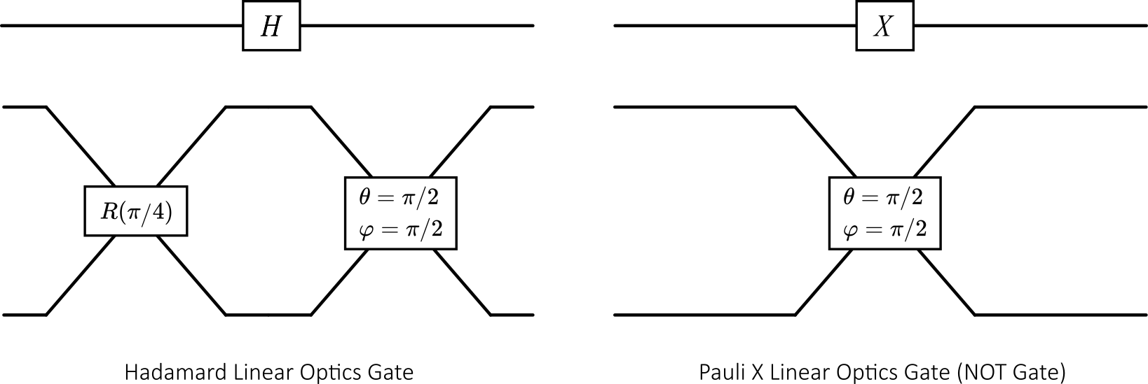
Since any two SU(2) rotations along orthogonal rotating axes can generate arbitrary rotations in the Bloch sphere, one can use a set of symmetric beam splitters and mirrors to realize an arbitrary SU(2) operators for QIP.

The following figures are examples of implementing a Hadamard gate and a Pauli-X gate (NOT gate) by using beam splitters and mirrors:

For further reading on LQOC & KLM, I would recommend these two papers:

Efficient Linear Optics Quantum Computation (E. Knill, R. Laflamme and G. Milburn)
Linear optical quantum computing (Pieter Kok, W.J. Munro, Kae Nemoto, T.C. Ralph, Jonathan P. Dowling and G.J. Milburn)

Continuous-Variable model

Many physical systems are intrinsically continuous, with light being the prototypical example. Such systems reside in an infinite-dimensional Hilbert space, offering a paradigm for quantum computation which is distinct from the qubit model.

This continuous-variable model (CV) takes its name from the fact that the quantum operators underlying the model have continuous spectra. The CV model is a natural fit for simulating bosonic systems (electromagnetic field, harmonic oscillators, phonons, Bose-Einstein condensates, …) and for settings where continuous quantum operators (such as position or momentum) are present.

In quantum optics, an optical phase space is a phase space in which all quantum states of an optical system are described. Each point in the optical phase space corresponds to a unique state. For any such system, the plot of the quadratures (i.e position and momentum) against each other is called a phase diagram:

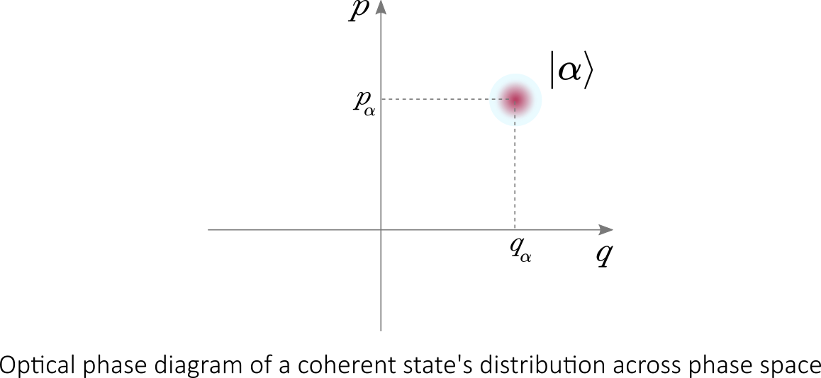
If the quadratures are functions of time then the optical phase diagram can show the evolution of a quantum optical system with time.

When discussing the quantum theory of light, it is very common to use an electromagnetic oscillator as a model. An electromagnetic oscillator describes an oscillation of the electric field. And since the magnetic field is proportional to the rate of change of the electric field, this too oscillates. Systems composed of such oscillators can be described by an optical phase space.

When quantized, such oscillators are described by quantum harmonic oscillators. which can be written in terms of creation and annihilation operators.

The Fock space is commonly used in quantum mechanics to construct the quantum states space of a variable number of identical particles from a single particle Hilbert space $H$ . It is the direct sum of the symmetric or antisymmetric tensors (depending on the bosonic or fermionic nature of the particles) in the tensor powers of a single-particle Hilbert:

$\displaystyle F_v = \bigoplus_{n=0}^\infty S_v H^{\otimes n}$

The creation operator $\hat{a}^\dagger$ acts on the Fock space, changing a $N$ particles state into a $N+1$ particles state. In the case of bosons, the $\hat{a}^\dagger$ operator creates a particle in state $i$ such as

$\displaystyle \hat{a}_i^\dagger | N_1,N_2, \cdots, N_i, \cdots \rangle = \sqrt{N_i + 1} |N_1, N_2, \cdots, N_{i+1},\cdots\rangle$

Conversely, the annihilation operator $\displaystyle \hat{a}$ acts on the Fock space, changing a $N$ particles state into a $N-1$ particles state. For bosonic states:

$\displaystyle \hat{a}_i^| N_1,N_2, \cdots, N_i, \cdots \rangle = \sqrt{N_i} |N_1, N_2, \cdots, N_{i-1},\cdots\rangle$

The number operator $N$ is defined as $N = \hat{a}^\dagger \hat{a}$ , leading to the following canonical commutation relations:

$[a,\hat{a}^\dagger] = 1$
$[N,\hat{a}^\dagger] = \hat{a}^\dagger$
$[N,\hat{a}] = -\hat{a}$

The quadrature operators can be defined in terms of creation an annihilation operators:

$\displaystyle \hat{x} \propto \sqrt{\frac{\hbar}{2}} (\hat{a} + \hat{a}^\dagger)$
$\displaystyle \hat{p} \propto -i \sqrt{\frac{\hbar}{2}} (\hat{a} - \hat{a}^\dagger)$
with $\displaystyle [\hat{x} , \hat{p}] = i \hbar$

The dichotomy between qubit and CV systems is perhaps most evident in the basis expansions of quantum states. For qubits, a discrete set of coefficients is used whereas CV systems have a continuum:

qubit: $\displaystyle |\psi\rangle = \alpha |0\rangle + \beta |1\rangle$
qumode: $\displaystyle |\psi\rangle = \int dx\; \psi(x) |x\rangle$

The following table draws a comparison of CV quantum computation with the qubit model:

	qubit model	Continuous-Variable model
Basic element	qubits	qmodes
Relevant operators	Pauli operators $\sigma_x, \sigma_y, \sigma_z$	Quadrature operators $\hat{x},\hat{p}$ and creation-annihilation operators $\hat{a}^\dagger, \hat{a}$
Common states	Pauli eigenstates $\|0\rangle, \|1\rangle, \cdots$	Coherent states $\|\alpha\|\rangle$ , Squeezed states $\|z\rangle$ , Number states $\|n\rangle$
Common gates	Phase Shift, Hadamard, CNOT, Pauli, …	Rotation, Displacement, Squeezing, Beam Splitter, …
Common measurements	Pauli-basis measurements $\|0\rangle \langle 0\|, \|1\rangle\langle 1\|, \cdots$	Homodyne, Heterodyne, Photon-counting $\|n\rangle \langle n\|$

Note: qubit-based computations can be embedded into the CV picture, e.g., by using the Gottesman-Knill-Preskill embedding, so the CV model is as computationally powerful as its qubit counterparts.

The starting point is the vacuum state $|0\rangle$ . Other states can be created by evolving $|0\rangle$ according to:

$\displaystyle |\psi\rangle = \mathrm{exp}(-itH) |0\rangle$

where $H$ is a bosonic Hamiltonian. States where the Hamiltonian is at most quadratic in the operators $\hat{x}$ and $\hat{p}$ are called Gaussian. Typically, for a one-dimensional harmonic oscillator, the Hamiltonian of the particle is given by:

$\displaystyle H = \frac{p^2}{2m} + \frac{1}{2}m\omega^2 x^2$

Solving Schrödinger’s equation $H|\psi\rangle = E|\psi\rangle$ leads indeed to a Gaussian ground state

$\displaystyle \psi_0 (x) = \Big( \frac{m\omega}{\pi\hbar}\Big)^{\frac{1}{4}}\; e^{-m\omega x^2/ 2\hbar}$

The displacement gives the center of the Gaussian, while the squeezing determines the variance and rotation of the distribution.

Of course, complementary to (continuous) Gaussian states are the discrete Fock states. Let’s introduce the eigenstate $|n\rangle$ of the number operator $N = \hat{a}^\dagger \hat{a}$ . Each Gaussian state can be expanded in the number state basis. For example, coherent states $|\alpha\rangle$ have the form:

$\displaystyle |\alpha\rangle = \mathrm{exp}\Big( -\frac{|\alpha|^2}{2}\sum_{n=0}^{\infty}\frac{\alpha^2}{\sqrt{n!}}\Big) |n\rangle$

Continuous-Variable gates

Unitary operations can always be associated with a generating Hamiltonian $H$

$\displaystyle U = \mathrm{exp}(-itH)$

A CV quantum computer is said to be universal if it can implement with a finite number of steps any unitary which is polynomial in the annihilation / creation operator. Two kinds of universal gates can be distinguished:

Gaussian gates: these are gates that are quadratic, such as displacement, rotation, squeezing, and beam splitter gates. These are equivalent to the Clifford quantum gates from the qubit model (Hadamard gates, controlled NOT gates, Phase Gate);
Non-Gaussian gates: these are gates which are of degree 3 or higher, e.g., the cubic phase gate.

The following table lists a few fundamental CV gates :

Gate	Unitary	Symbol
Displacement	$\displaystyle D_i(\alpha)=\mathrm{exp}(\alpha \hat{a}^\dagger_i - \alpha^* \hat{a}_i)$
Rotation	$\displaystyle R_i(\phi)=\mathrm{exp}(i\phi N_i)$
Squeezing	$\displaystyle S_i(z)= \mathrm{exp} \Big( \frac{1}{2} (z^* \hat{a}_i^2 - z\hat{a}^{\dagger 2}_i) \Big)$
Beam Splitter	$\displaystyle B_{i,j}(\theta, \phi)= \mathrm{exp} \Big( \theta (e^{i\phi}\hat{a}_i^{\dagger} \hat{a}_j - e^{-i\phi} \hat{a}_i \hat{a}_j^{\dagger} ) \Big)$
Cubic Phase	$\displaystyle V_i(\gamma)= \mathrm{exp}\big( i \frac{\gamma}{6}\hat{x}^3_i \big)$

Software architecture for photonic quantum computing

The Strawberry Fields software platform is a full-stack Python library for designing, simulating, and optimizing Continuous Variable quantum optical circuits.

The following sketch outlines its key elements :

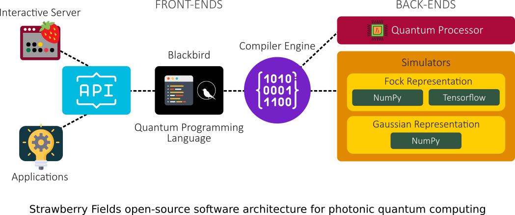
The platform consists of three main components:

an API for quantum programming based a programming language named Blackbird;
a suite of three virtual quantum computer backends, built in NumPy and Tensorflow, each targeting specialized uses (Optimization, Quantum Machine Learning, …);
an engine which can compile Blackbird programs on various backends, including the three built-in simulators, and – in the near future – photonic quantum information processors.

The frontend encompasses the Strawberry Fields Python API and the Blackbird quantum programming language. These elements provide access points for users to design quantum circuits.

Blackbird is a quantum assembly language, capable of representing the basic continuous-variable (CV) states, gates, and measurements. There are four main types of operations:

State preparation;
Gate application;
Measurements;
Adding and removing subsystems that these operations act on.

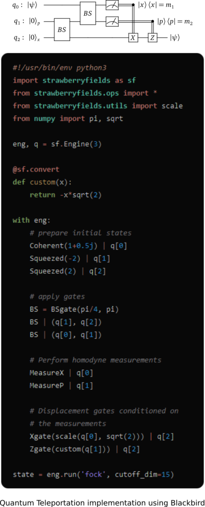
The following example shows an implementation of Quantum Teleportation with the Blackbird quantum programming language:

For a backend, the engine can target one of the included quantum computer simulators:

Gaussian Representation (using Numpy)
Fock Representation (using Numpy and Tensorflow)

When CV quantum processors will become available, the engine will also build and run circuits on these devices.

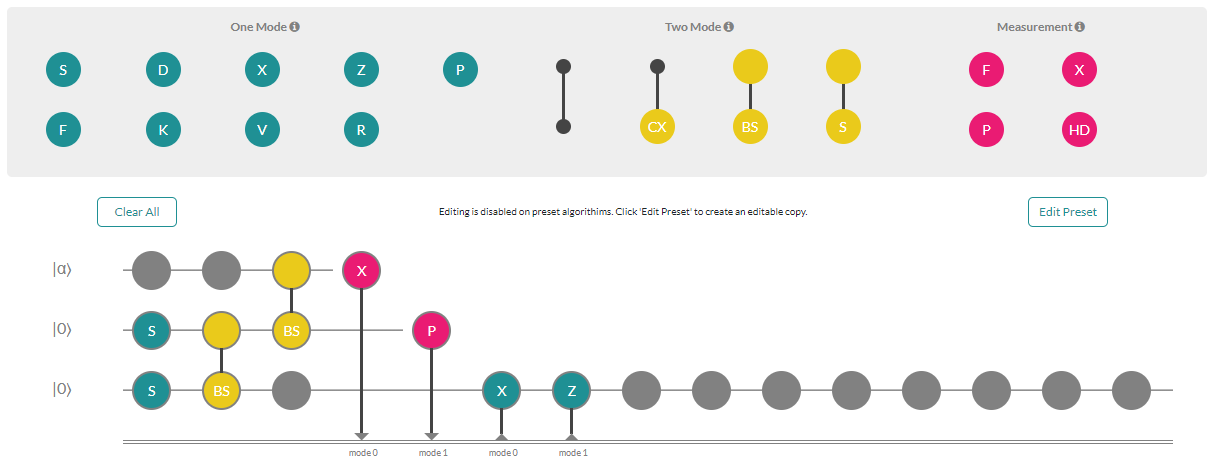
Applications, such as the Strawberry Fields Interactive website, can be built by leveraging the frontend API. The following screenshot demonstrates how to perform quantum teleportation using Strawberry Fields Interactive :

More information on the platform is available here: https://www.xanadu.ai/software/

Yes, the authors are obviously fans of The Beatles 🙂

Note: to speedup the writing process, a few paragraphs and illustrations of this post are based selected papers and Wikipedia articles on the subject of LQOC as well as a few excerpts from the Strawberry Fields Open-source software for photonic quantum computing documentation.

Leave a Reply Cancel reply