Building a quantum device in the real world means having to deal with errors: any qubit stored unprotected or transmitted through a communications channel will inevitably come out changed.
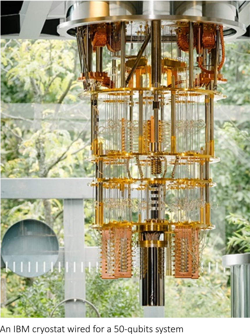
To be protected, quantum devices have to be kept at extremely cold temperatures (a few milikelvins) and shielded from electromagnetic radiation.
Quantum error correction is used in quantum computing to protect quantum information from errors due to decoherence and quantum noise.
It is essential if one is to achieve fault-tolerant quantum computation that can deal not only with noise on stored quantum information, but also with faulty quantum gates, faulty quantum preparation, and faulty measurements.
In classical computing, if one wants to protect a bit against errors, it can often suffice is to store the information multiple times.
Let 

We have here a simple repetition code that protects against any one bit flip error. That is, if any of the three bits are flipped, then we can recover the state of the logical bit by taking a majority vote.
Classical error correcting codes use a syndrome measurement to diagnose which error corrupts an encoded state. We then reverse an error by applying a corrective operation based on the syndrome.
No-cloning theorem
In physics, the no-cloning theorem states that it is impossible to create an identical copy of an arbitrary unknown quantum state. It proves the impossibility of a simple perfect non-disturbing measurement scheme. Conversely, the no-deleting theorem is the time-reversed dual to this theorem. It states that, given two copies of some arbitrary quantum state, it is impossible to delete one of the copies.
The no-cloning theorem has profound implications in quantum computing. It implies that if we measure each individual qubit and take a majority vote by analogy to classical code above, then we have lost the precise information that we are trying to protect.
At first sight, the no-cloning theorem seems to present an obstacle to formulating a theory of quantum error correction.
It is nevertheless possible to spread the information of one qubit onto a highly entangled state of several qubits. Peter Shor first discovered this method of formulating a quantum error correcting code by storing the information of one qubit onto a highly entangled state of nine qubits.
QEC (Quantum Error Correction)
Just like classical error correction, QEC also employs syndrome measurements. We perform a multi-qubit measurement that does not disturb the quantum information in the encoded state but retrieves information about the error.
A syndrome measurement can determine whether a qubit has been corrupted, and if so, which one. What is more, the outcome of this operation (the syndrome) tells us not only which physical qubit was affected, but also, in which of several possible ways it was affected.
The syndrome measurement tells us as much as possible about the error that has happened, but nothing at all about the value that is stored in the logical qubit—as otherwise the measurement would destroy any quantum superposition of this logical qubit with other qubits in the quantum computer.
In most codes, the effect is either a bit flip, or a sign (of the phase) flip, or both (corresponding to Pauli X, Z, and Y matrices):

Let’s get back to the idea of encoding repeated data bits and let’s define


Now, let’s define the following bit-flip errors E and their actions :
| Errors (E) | ") |
") |
 |
 |
 |
 |
 |
 |
 |
 |
 |
 |
 |
 |
Let’s pause a moment to focus en Pauli measurement. The Pauli Z-matrix is defined as:

The Pauli-Z matrix clearly has two eigenvectors 

Thus if we measure the qubit and obtain
This process is referred to in the language of Pauli measurements as “measuring Pauli Z” and is equivalent to performing a computational basis measurement.
In that spirit, we will define 


For example, if we measure 

On the other hand, consider measuring 


Note that 


For clarity sake, we now repeat the previous table, but we added the results of measuring 
| Errors (E) | |
|
Result of |
Result of |
|
|
|
+ | + |
|
|
|
– | + |
|
|
|
– | – |
|
|
|
+ | – |
Thus, the results of the two measurements uniquely determines which bit-flip error occured, but without revealing any information about which state we encoded. These results are a syndrome, and refer to the process of mapping a syndrome back to the error that caused it as recovery.
In particular, we emphasize that recovery is a classical inference procedure which takes as its input the syndrome which occured, and returns a prescription for how to fix any errors that may have occured.
Bear in mind that the error channel may induce either a bit flip, a sign flip, or both.
It is possible to correct for both types of errors using one code, and the Shor code does just that. In fact, the Shor code corrects arbitrary single-qubit errors.
The Shor code, encodes 1 logical qubit in 9 physical qubits and can correct for arbitrary errors in a single qubit:

The insight that we can describe measurements in quantum error correction that act the same way on all code states, is the essence of the stabilizer formalism.
To go beyond this introduction, you might be interested in reading Daniel Gottesman’s 2009 paper “An Introduction to Quantum Error Correction and Fault-Tolerant Quantum Computation”.
Quantum Error Correcting Codes in Q#
To conclude this introduction, we will list the user-defined type used to specify error correcting codes, as provided by the Q# canon (excerpt from Q# documentation):
- LogicalRegister (= Qubit[]): Denotes that a register of qubits should be interpreted as the code block of an error-correcting code.
- Syndrome (= Result[]): Denotes that an array of measurement results should be interpreted as the syndrome measured on a code block.
- RecoveryFn (= (Syndrome -> Pauli[])): Denotes that a classical function should be used to interpret a syndrome and return a correction that should be applied.
- EncodeOp (= ((Qubit[], Qubit[]) => LogicalRegister)): Denotes that an operation takes qubits representing data along with fresh ancilla qubits in order to produce a code block of an error-correcting code.
- DecodeOp (= (LogicalRegister => (Qubit[], Qubit[]))): Denotes than an operation decomposes a code block of an error correcting code into the data qubits and the ancilla qubits used to represent syndrome information.
- SyndromeMeasOp (= (LogicalRegister => Syndrome)): Denotes an operation that should be used to extract syndrome information from a code block, without disturbing the state protected by the code.
Finally, the canon provides the QECC (Quantum Error Correcting Code) type to collect the other types required to define a quantum error-correcting code.
Notice that the QECC type does not include a recovery function. This allows us to change the recovery function that is used in correcting errors without changing the definition of the code itself; this ability is in particular useful when incorporating feedback from characterization measurements into the model assumed by recovery.
Once a code is defined in this way, we can use the Recover operation to recover from errors.
Aside from the bit-flip code, the Q# canon is provided with implementations of the five-qubit perfect code, and the seven-qubit code, both of which can correct an arbitrary single-qubit error.
Note: to speedup the writing of this post, a few paragraphs and illustrations are based on wikipedia’s entries on quantum error correction and MS Quantum Development Kit documentations.