On quantum computing – Quantum Bits

Quantum computing as made the headlines recently. At IBM’s inaugural Index Developer Conference held in San Francisco, the company showed off its latest prototype: a quantum computing rig housing 50 qubits, one of the most advanced machines currently in existence.

Google Quantum AI Lab announced Bristlecone, its new quantum processor, at the annual American Physical Society meeting in Los Angeles. This gate-based superconducting system is to provide a testbed for research into system error rates and scalability of our qubit technology, as well as applications in quantum simulation, optimization, and machine learning.

Microsoft released the first version of its quantum development kit and a new quantum computing programming language (Q#) last December. On february, the company released an update that adds support for quantum development on macOS and GNU/Linux. Both the Q# language, MS’s quantum simulator, will run on these platforms in addition to Windows.

It’s been almost 10 years (!) since I published a small post about quantum information … that is still lacking a follow up. And, unfortunately, there was only very little on that subject in the series of posts on hidden realities I published a couple of years ago :

On hidden realities (part 1) – Many-worlds interpretation of quantum mechanics
On hidden realities (part 2) – Space-time geometries and dynamics
On hidden realities (part 3) – Higher dimensional universes
On hidden realities (part 4) – Holographic principle
On hidden realities (part 5) – Simulated reality

So, I think it’s about time to get (a little) deeper about the basis of quantum computing !

What is quantum computing ?

In simple terms, a quantum computer is any device that uses quantum mechanical phenomena, such as superposition or entanglement to perform calculations or manipulate data.

Whereas common computing requires the data to be encoded into binary digits (known as bits), each of which is always in one of two definite states (0 or 1), quantum computation uses quantum bits (known as qubits), which are superpositions of quantum states.

Quantum computing is still in its infancy. Experiments have been carried out in which operations are executed on a very small number of quantum bits (Google’s Bristlecone 72 qubits processor being the record as of 2018). Practical and theoretical research are carried on, in effort to develop quantum computers for civilian, business, trade, environmental and security purposes, such as cryptanalysis.

Quantum computing typically aims at solving certain classes of problems (like integer factorization) quicker than any classical computers or simulating multi-body quantum systems. Indeed, there exist quantum algorithms, such as Simon’s algorithm, that run faster than any possible probabilistic classical algorithm.

It is worth noting that a classical computer could in principle (with exponential resources) simulate a quantum algorithm, as quantum computation does not violate the Church–Turing thesis. On the other hand, quantum computers may be able to efficiently solve problems which are not practically feasible on classical computers.

Quantum computing is of great importance for cryptography and cryptanalysis. Typically, RSA public key encryption relies on the difficulty of factoring large integers. It is conjectured that factorization is impossible to do efficiently with a classical computer. Shor’s factoring algorithm for quantum computers would render this encryption method useless.

Quantum information

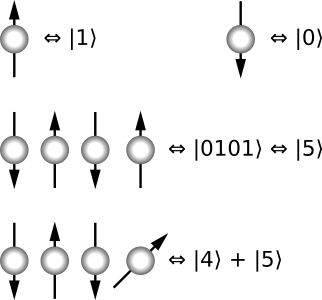
In quantum computing, a quantum bit (or qubit) is a unit of information. It is modeled as a common two-state quantum-mechanical system.

In a classical system, a bit would have to be either in one state or the other. In a quantum system, a qubit can be a superposition of both states at the same time, a property that is fundamental to quantum computing.

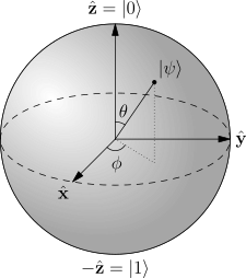
Let’s enter the realm of quantum mechanics. As we have seen, a quantum state can be mathematically described an element of a Hilbert vector space. Following Dirac’s notation, a quantum state (or ket) will denoted as $|\psi\rangle$ .

Let’s introduce the following vectors $|0\rangle = \begin{bmatrix}1 \\ 0 \end{bmatrix}$ and $|1\rangle = \begin{bmatrix}0 \\ 1 \end{bmatrix}$ .

A pure state qubit would be represented as a linear combination of $|0\rangle$ and $|1\rangle$ :

$|\psi\rangle = \alpha |0\rangle + \beta |1\rangle$ where $\alpha$ and $\beta$ are probability amplitudes.

Operators act on quantum states. More specifically, observables are self-adjoint hermitian operators.

Classical computation

Now, let’s get back for a moment to non-quantum computing. Computation is done by means of an algorithm, which can be thought of as a set of instructions for solving a specific problem.

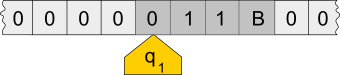
Around 1936-37, the great mathematician, logician, computer scientist, cryptanalyst, philosopher, and theoretical biologist Alan Turing devised a hypothetical machine that could execute any algorithm called … a Turing Machine.

A Turing machine consists of:

A tape, divided into cells. Each cell contains a symbol from some finite alphabet. The tape is assumed to be arbitrarily extendable to the left and to the right.
A head, that can read and write symbols on the tape and move the tape left and right one (and only one) cell at a time.
A state register that stores the (finate) state of the machine.
A (finite) table of instructions that, given the state (q_i) the machine is currently in and the symbol (a_j) it is reading on the tape (symbol currently under the head), tells the machine what to do: erase or write a symbol, move the head, …

Programs are defined by a set of instructions. An instruction can be written as T:(q,a) → (q’,a’,d), where q is the current state and q’ is the final state of the head, a is the symbol in the cell, a’ is the symbol to be written, d is the direction the head will move.

The input is the initial state of the Turing machine.The output of a Turing machine is the final state of the Turing machine (if any). For a Turing machine it is impossible to know for all inputs whether the control head will reach a halting state or not. This is the known as the halting problem.

A Turing machine that is able to simulate any other Turing machine is called a universal Turing machine. A more mathematically oriented definition with a similar “universal” nature was introduced by Alonzo Church, whose work on lambda calculus intertwined with Turing’s in a formal theory of computation known as the Church–Turing thesis.

The thesis conjectures that any function whose values can be computed by an algorithm can be computed by a Turing machine, and therefore that if any real-world computer can simulate a Turing machine, it is Turing equivalent to a Turing machine.

These principles are considered to be the origin of the idea of a stored-program computer used by John von Neumann in 1946 for the “Electronic Computing Instrument” that now bears his name: the von Neumann architecture.

Logic gates

Logic gates is an idealized or physical device implementing a Boolean function. A logic gate performs a logical operation on one or more binary inputs and produces a binary output. In any computation, a circuit (made of logic gates) can be represented as mapping a n-bit input to a m-bit output.

The following table lists such logic gates:

NOT	$\overline{A}$	Negation
AND	$A \cdot B$	Conjunction
OR	$A + B$	Disjunction
NAND	$\overline{A \cdot B}$	Alternative denial
NOR	$\overline{A + B}$	Joint denial
XOR	$A \oplus B$	Exclusive Or
XNOR	$\overline{A \oplus B}$	Biconditional

These gates can be expressed as linear operators.

The logic gate “NOT” can trivially be represented as a 2 x 2 matrix:

$\textsf{NOT} = \begin{bmatrix} 0 & 1 \\ 1 & 0 \end{bmatrix}$

$\textsf{NOT}|1\rangle = \begin{bmatrix} 0 & 1 \\ 1 & 0 \end{bmatrix} \begin{bmatrix}0 \\ 1 \end{bmatrix}=\begin{bmatrix}1 \\ 0 \end{bmatrix}=|0\rangle$

As an example, one can build a circuit of logic gates in order to process binary additions:

Quantum computation

Quantum bits can be manipulated in a manner analogous to the logic gates and circuit models of classical computation.

We have seen, that for a single qubit (2-level system):

$|\psi\rangle = \alpha |0\rangle + \beta |1\rangle$ or, simply $|\psi\rangle = \begin{bmatrix} \alpha \\ \beta \end{bmatrix}$

How can it be extended to a 2-qubit system ?

First, let’s define two qubits:

$|\psi_1\rangle = \begin{bmatrix} \alpha_1 \\ \beta_1 \end{bmatrix}$ and $|\psi_2\rangle = \begin{bmatrix} \alpha_2 \\ \beta_2 \end{bmatrix}$

A 2-qubit can be represented as a tensor product :

$|\psi_1 \psi_1\rangle = |\psi_1\rangle \otimes |\psi_2\rangle$ or $|\psi_1 \psi_1\rangle = \begin{bmatrix} \alpha_1 \alpha_2 \\ \alpha_1 \beta_2 \\ \beta_1 \alpha_2 \\ \beta_1 \beta_2\end{bmatrix}$

In order to represent a 2-qubit system, a 4-dimensional vector is needed.

A basis for a 2-qubit system can be written as the tensor products of the individual qubit’s

basis vectors:

$| 0 0 \rangle = | 0 \rangle \otimes | 0 \rangle$
$| 0 1 \rangle = | 0 \rangle \otimes | 1 \rangle$
$| 1 0 \rangle = | 1 \rangle \otimes | 0 \rangle$
$| 1 1 \rangle = | 1 \rangle \otimes | 1 \rangle$

A quantum computer with a given number of qubits is fundamentally different from a classical computer composed of the same number of classical bits.

Representing the state of an n-qubit system requires (on a classical computer) the storage of 2ⁿ (complex) numbers, whereas to characterize the state of a classical n-bit system, it is sufficient to store only n numbers.

A quantum computer may be thought of as a collection of n-qubits called a quantum register. One n-qubit quantum register has a basis of 2ⁿ allowed states, and any state of the quantum computer is in a superposition of these states.

At first sight, it would seem that qubits can hold exponentially more information than their classical counterparts. But one must mustn’t overlook the fact that the qubits are only in a probabilistic superposition of all of their states.

This means that when the final state of the qubits is measured, they will only be found in one of the possible configurations they were in before the measurement. Quantum mechanically speaking, it is generally incorrect to think of a system as being in one particular state before the measurement.

Quantum entanglement

An important distinguishing feature between a qubit and a classical bit is that multiple qubits can exhibit quantum entanglement. This is a nonlocal property that allows a set of qubits to express higher correlation than is possible in classical systems.

Quantum entanglement is a physical phenomenon which occurs when pairs or groups of particles are generated or interact in ways such that the quantum state of each particle cannot be described independently of the state of the other(s), even when the particles are separated by a large distance—instead, a quantum state must be described for the system as a whole.

Let’s consider 2-qubit systems. A 2-qubit state is said to be separable if it can be written as the tensor product of two 1-qubit states. Example:

$\displaystyle | \psi_s \rangle = \frac{1}{\sqrt{2}} \big( | 01 \rangle +| 11 \rangle \big) = \frac{1}{\sqrt{2}} \big( | 0 \rangle +| 1 \rangle \big) \otimes | 1 \rangle$

A 2-qubit state is entangled otherwise. Example:

$\displaystyle | \psi_e \rangle = \frac{1}{\sqrt{2}} \big( | 00 \rangle +| 11 \rangle \big)$

This last state is also known as a Bell state. In this state, there are equal probabilities ( $|\frac{1}{\sqrt{2}}|^2=\frac{1}{2}$ ) of measuring either

| 00 \rangle

Now, let’s imagine that these entangled 2-qubits are separated: one each given to Alice and Bob. Alice makes a measurement of her qubit, obtaining either

| 0 \rangle

| 1 \rangle

Because of the qubits’ entanglement, Bob must now get exactly the same measurement as Alice : if she measures a

| 0 \rangle

, Bob must measure the same, as

| 00 \rangle

is the only state where Alice’s qubit is a

| 0 \rangle

Entanglement also allows multiple states (such as the Bell state mentioned above) to be acted on simultaneously, unlike classical bits that can only have one value at a time. Entanglement is a necessary ingredient of any quantum computation that cannot be done efficiently on a classical computer. Many of the successes of quantum computation and communication, such as quantum teleportation and superdense coding, make use of entanglement, suggesting that entanglement is a resource that is unique to quantum computation.

Quantum logic gates

A quantum logic gate can operate on a qubit. Mathematically speaking, the qubit undergoes a unitary transformation. Unitary transformations correspond to rotations of the qubit vector in the Bloch sphere.

Prerequisites for quantum computation are:

Being able to prepare system in a well defined initial state: $| \psi_i \rangle = | 011 \dots 101 \rangle$
Being able to manipulate the quantum state via unitary transformations: $| \psi_f \rangle = \textbf{U} | \psi_i \rangle$
Be able to measure the final states of each qubit : $| \psi_f \rangle = | 001 \dots 011 \rangle$

The most common quantum gates operate on spaces of one or two qubits, just like the common classical logic gates operate on one or two bits.

As matrices, quantum gates can be described by 2ⁿ x 2ⁿ sized unitary matrices, where $n$ is the number of qubits the gate acts on.

The Hadamard gate is a 1-qubit rotation, mapping the qubit-basis states $| 0 \rangle$ and $| 1 \rangle$ to two superposition states with equal weight of the computational basis states $| 0 \rangle$ and $| 1 \rangle$ .

It is commonly defined as:

$\displaystyle H = \frac{ | 0 \rangle + | 1 \rangle } { \sqrt{2} } \langle 0 | + \frac{ | 0 \rangle - | 1 \rangle } { \sqrt{2} } \langle 1 |$ ,

so that gate operations are:

$\displaystyle H | 0 \rangle = \frac{1}{\sqrt{2}} | 0 \rangle + \frac{1}{\sqrt{2}} |1 \rangle$
$\displaystyle H | 1 \rangle = \frac{1}{\sqrt{2}} | 0 \rangle - \frac{1}{\sqrt{2}} |1 \rangle$
$\displaystyle H \Big( \frac{1}{\sqrt{2}} | 0 \rangle + \frac{1}{\sqrt{2}} | 1 \rangle \Big) = | 0 \rangle$
$\displaystyle H \Big( \frac{1}{\sqrt{2}} | 0 \rangle - \frac{1}{\sqrt{2}} | 1 \rangle \Big) = | 1 \rangle$

or, using $| 0 \rangle$ and $| 1 \rangle$ as a representation basis:

$\displaystyle H = \frac{1}{\sqrt{2}} \begin{bmatrix} 1 & 1 \\ 1 & -1 \end{bmatrix}$

One application of the Hadamard gate to either a 0 or 1 qubit will produce a quantum state that, if observed, will be a 0 or 1 with equal probability (as seen in the first two operations). This is exactly like flipping a fair coin in the standard probabilistic model of computation.

However, if the Hadamard gate is applied twice in succession (as is effectively being done in the last two operations), then the final state is always the same as the initial state. This would be like taking a fair coin that is showing heads, flipping it twice, and it always landing on heads after the second flip.

It is a crucial part of Grover’s algorithm and Shor’s algorithm in quantum computing.

There are many other quantum gates that can be defined, such as :

Hadamar H gate		Definition (wikipedia)
Pauli-X gate (NOT gate)		Definition (wikipedia)
Square root of NOT gate		Definition (wikipedia)
Swap (S) gate		Definition (wikipedia)
Square root of Swap gate (√S)		Definition (wikipedia)
Controlled gates (here, a C-NOT gate)		Definition (wikipedia)

Note: this list is not exhaustive.

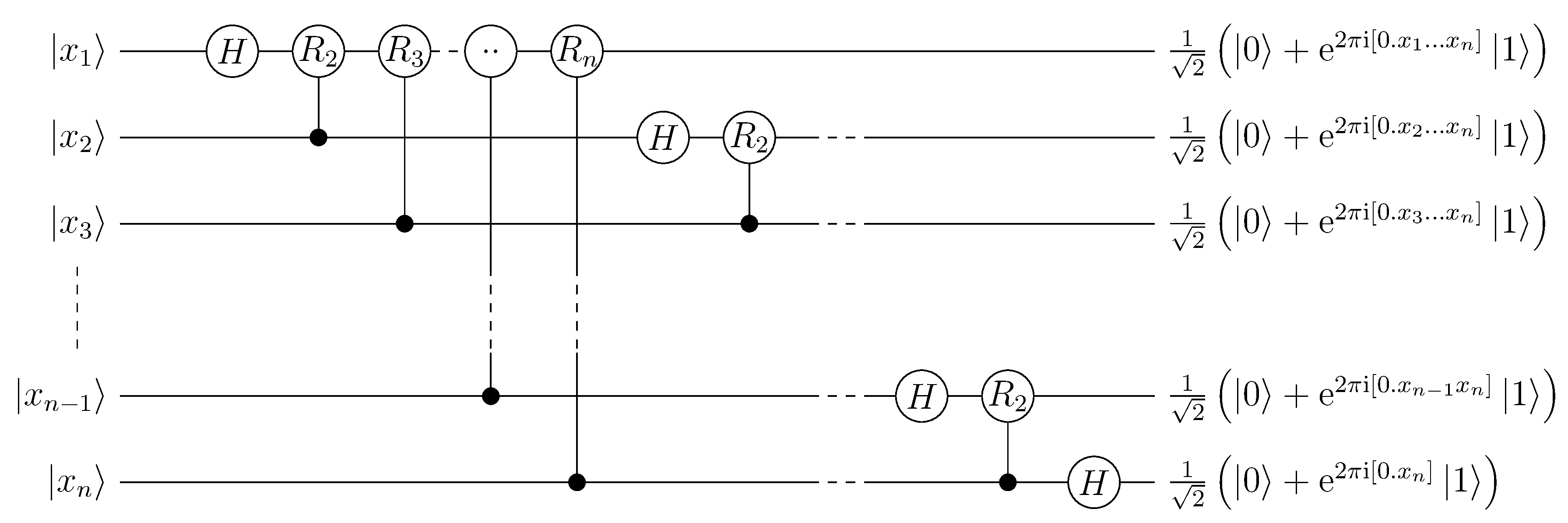
In quantum information theory, a quantum circuit is a model in which a computation is a sequence of quantum gates.

The following diagram is a typical quantum circuit, built on Hadamar gates and controlled gates, used for Quantum Fourier Transforms (QFT):

Such quantum logic gate can be implemented via quantum devices, such as C-NOT gates built using trapped ions (see this NIST paper for example).

Deutsch(–Jozsa) algorithm

The Deutsch–Jozsa algorithm is a quantum algorithm, proposed by David Deutsch and Richard Jozsa in 1992 (and generalizing 1985’s work from David Deutsch).

It is specifically designed to be easy for a quantum algorithm and hard for any classical algorithm. The motivation is to show a black box problem that can be solved efficiently by a quantum computer with no error, whereas a deterministic classical computer would need exponentially many queries to the black box to solve the problem.

In the Deutsch-Jozsa problem, we are given a black box quantum computer known as an oracle that implements a function $f:\{0,1\}^n \to \{0,1\}$ takes n-digit binary values as input and produces either a 0 or a 1 as output for each such value.

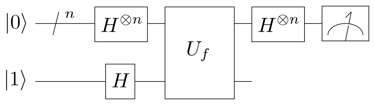
The task is to determine if $f$ is constant (0 on all outputs or 1 on all outputs) or balanced (returns 1 for half of the input domain and 0 for the other half) by using the oracle.

For the Deutsch–Jozsa algorithm to work, the oracle computing $f(x)$ from $x$ has to be a quantum oracle which doesn’t decohere $x$ . It also mustn’t leave any copy of $x$ lying around at the end of the oracle call.

The following diagram illustrates Deutsch-Jozsa algorithm’s quantum circuit, using Hadamar quantum gates:

Shor’s Algorithm

Shor’s algorithm, named after mathematician Peter Shor, is a quantum algorithm formulated in 1994. Unlike Deutsch’s, which is of great historical importance but without practical applications, Shor’s algorithm solves a practical problem: given an integer N, find its prime factors.

The following diagram illustrates the quantum subroutine of Shor’s algorithm:

It is based on Hadamar gates and QFT’s. On a quantum computer, to factor an integer N, Shor’s algorithm runs in polynomial time. This is substantially faster than the most efficient known classical factoring algorithm (the general number field sieve), which works in sub-exponential time.

If a quantum computer with a sufficient number of qubits could operate without succumbing to quantum noise and quantum decoherence phenomena, Shor’s algorithm could be used to break public-key cryptography schemes (such as the widely used RSA scheme).

RSA is based on the assumption that factoring large numbers is computationally intractable. So far as is known, this assumption is valid for classical (i.e. non-quantum) computers. No classical algorithm is known that can factor in polynomial time.

However, Shor’s algorithm shows that factoring is efficient on an ideal quantum computer, so it may be feasible to defeat RSA by constructing a large quantum computer. It was also a powerful motivator for the design and construction of quantum computers and for the study of new quantum computer algorithms.

It has also facilitated research on new cryptosystems that are secure from quantum computers, collectively called post-quantum cryptography.

Quantum supremacy

Based on ideas from Richard Feynman (and other’s), renown physisit John Preskill popularized the term “quantum supremacy” to refer to the hypothetical speedup advantage that a quantum computer would have over a classical computer in a given field.

And actually, Shor’s algorithm for factoring integers provides a superpolynomial speedup over the best known classical algorithm.

However, practically speaking, quantum computers are much more susceptible to errors than classical computers due to decoherence and to quantum noise. It is not known (yet) how the resources needed for quantum error correction will scale with the number of qubits.

One of the greatest challenges is controlling or removing quantum decoherence. This means isolating the system from its environment as interactions with the external world cause the system to decohere. However, other sources of decoherence also exist. Examples include the quantum gates, and the lattice vibrations and background thermonuclear spin of the physical system used to implement the qubits.

Decoherence is irreversible, as it is effectively non-unitary, and is usually something that should be highly controlled, if not avoided. Currently, some quantum computers require their qubits to be cooled to 20 millikelvins in order to prevent significant decoherence.

It was also pointed out that a 400-qubit computer would even come into conflict with the cosmological information bound implied by the holographic principle (which could be a property of quantum gravity).

Like the “AI singularity”, “Quantum supremacy” is not that well defined: reaching “supremacy” is always linked to a given field.

This is actually not a surprise since we are dealing with subjects on the fringe of our knowledge. Since the term is often misused for clickbait articles, I refrain myself as much as possible from using this term: quantum computational advantage seems (for me) better suited and more objective.

Sometimes, it is extremely hard to even prove that a given device has achieved quantum speedup.

But it might be practically reached on particular subjects, such as cryptography, namely because of the effectiveness of Shor’s algorithm (on ideal quantum computers) and because it seems were are close to reach availability of devices able to manage large qubits registers.

On this particular field, risks are important enough for security and privacy to strongly promote and evaluate post-quantum cryptography (like lattice-based cryptography).

Quantum information science

As a conclusion, let’s enlarge our vision. Quantum information, as a science, is an area of study based on the idea that information science depends on quantum effects in physics. It includes theoretical issues in computational models as well as more experimental topics in quantum physics (including what can and cannot be done with quantum information).

It is a large field of research, which of course includes quantum computing, but also include

Quantum error correction
Quantum information theory
Quantum complexity theory
Quantum cryptography and its generalization to quantum communication
Quantum communication complexity
Quantum entanglement, as seen from an information-theoretic point of view
Quantum dense coding
Quantum teleportation
Quantum simulation
…

Hopefully, I’ll get some times (soon ?) to write a few notes on these tremendously interesting subjects 😉

Note: to speedup the writing of this long long long overdue post, a few paragraphs and illustrations are based on wikipedia’s entries on quantum computing, which are well written, though sometimes a bit technical for an introduction post.

Leave a Reply Cancel reply