Having fun with Bell states and Q#

In a previous post, we introduced the basic concepts of quantum computing, during which quantum entanglement, Bell states and usual quantum gates such as Hadamard’s or Pauli’s were quickly addressed.

Today, we’re going to explore some of these concepts and start having fun with quantum programming to illustrate these ideas.

Quantum entanglement

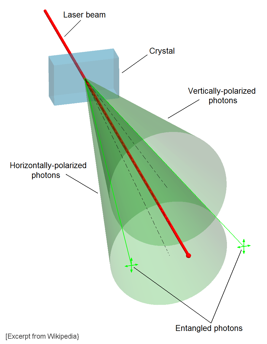
Quantum entanglement is a phenomenon which occurs when pairs (or groups) of particles are generated (or interact) in such a way that the quantum state of each particle cannot be described independently of the state of the other(s), even when the particles are separated by a large distance:  the quantum state must be described for the system as a whole.

Measurements of physical properties (position, momentum, spin, polarization …) performed on entangled particles are found to be correlated. Let’s imagine a pair of particles generated in such a way that their total spin is known to be zero.

Now, let’s imagine that one particle is found to have clockwise spin on a certain axis. Because they are entangled, the spin of the other particle, measured on the same axis, will be found to be counterclockwise !

This behavior gives rise to paradoxical effects: any measurement of a property of a particle can be seen as acting on that particle. In the case of entangled particles, such a measurement will be on the entangled system as a whole.

It seems to appear that one particle of an entangled pair “knows” what measurement has been performed on the other, and with what outcome, even though there is no known means for such information to be communicated between the particles, which at the time of measurement may be separated by any arbitrarily large distances (Einstein referring to it as “spooky action at a distance”).

EPR paradox

Such phenomena were the subject of a 1935 paper by Albert Einstein, Boris Podolsky, and Nathan Rosen (and several papers by Erwin Schrödinger) describing what came to be known as the EPR paradox.

This thought experiment aims at the Copenhagen interpretation (more precisely, at the wave function collapse). Resolutions of the paradox have important implications for the interpretation of quantum mechanics.

In quantum mechanics, a particle is described by a quantum state. This quantum state can be represented as a superposition (i.e. a linear combination) of basis states. In principle one is free to choose the set of basis states, as long as they span the space. If one chooses the eigenfunctions of the position operator as a set of basis functions, one speaks of a state as a wave function position space.

For a quick recap on bra-ket notations, inner products, operators, observables and all that jazz, please, have a look at this (old) post.

Let’s define the ket , representing a quantum state. The wave function (position space) can be defined as .

This wave function is interpreted as a (complex-valued) probability amplitude. The probabilities for the possible results of measurements made on the system are :

Quantum frameworks do not provide single measurement outcomes in a deterministic way. According to the understanding of quantum mechanics known as the Copenhagen interpretation, measurement causes an instantaneous collapse of the wave function describing the quantum system into an eigenstate of the observable that was measured.

Einstein was one of the most prominent opponent of the Copenhagen interpretation. In his view, quantum mechanics was incomplete. Commenting on this, other writers (such as John von Neumann and David Bohm) hypothesized that consequently there would have to be ‘hidden’ variables responsible for random measurement results.

The article that first brought forth these matters, “Can Quantum-Mechanical Description of Physical Reality Be Considered Complete?” was published in 1935 by Einstein, Podolsky, and Rosen (EPR). The paper prompted a response by Niels Bohr, which he published in the same journal, in the same year, using … the same title 🙂

Einstein had been skeptical of the Heisenberg uncertainty principle and the role of chance in quantum theory.

But the crux of this debate was not about chance, but something deeper:

• Is there one objective physical reality, which every observer sees from his own vantage? (Einstein’s view)
• Or does the observer co-create physical reality by the questions he poses with experiments? (Bohr’s view).

The EPR description involves “two particles, A and B, which interact briefly and then move off in opposite directions.” According to Heisenberg’s uncertainty principle, it is impossible to measure both the momentum and the position of particle B exactly. However, it is possible to measure the exact position of particle A. By calculation, therefore, with the exact position of particle A known, the exact position of particle B can be known. Alternatively, the exact momentum of particle A can be measured, so the exact momentum of particle B can be worked out.

EPR tried to set up a paradox to question the range of true application of quantum mechanics: quantum theory predicts that both values cannot be known for a particle, and yet the EPR thought experiment purports to show that they must all have determinate values.

Since 1972, experiments analogous to the one described in the EPR paper have been carried out, notably at the Saclay Nuclear Research Centre. These experiments appear to show that Einstein’s local realism idea is false, vindicating Bohr !

Bell’s theorem and experiments

The original EPR paradox challenges the prediction of quantum mechanics that it is impossible to know both the position and the momentum of a quantum particle. This challenge can however be extended to other pairs of physical properties

While EPR felt that the paradox showed that quantum theory was incomplete and should be extended with hidden variables, the usual modern resolution is to say that due to the common preparation of the two particles (for example the creation of an electron-positron pair from a photon) the property we want to measure has a well defined meaning only when analyzed for the whole system while the same property for the parts individually remains undefined.

Therefore, if similar measurements are being performed on the two entangled subsystems, there will always be a correlation between the outcomes resulting in a well defined global outcome i.e. for both subsystems together. However, the outcomes for each subsystem separately at each repetition of the experiment will not be well defined or predictable.

Note that this correlation does not imply any action of the measurement of one particle on the measurement of the other. Therefore it does not imply any form of (spooky) action at a distance or any violation of special relativity (effects propagating faster than light). This modern resolution eliminates the need for hidden variables, action at a distance or other structures introduced over time in order to explain the phenomenon.

In 1964, John Bell showed that the predictions of quantum mechanics in the EPR thought experiment are significantly different from the predictions of a particular class of hidden variable theories (the local hidden variable theories).

These differences, expressed using inequality relations known as “Bell’s inequalities”, are in principle experimentally detectable.

Bell’s theorem is a “no-go theorem” that draws an important distinction between quantum mechanics and the world as described by classical mechanics. Bell’s theorem rules out local hidden variables as a viable explanation of quantum mechanics (though it still leaves the door open for non-local hidden variables)

After the publication of Bell’s paper “On the Einstein Podolsky Rosen paradox”, a variety of experiments to test Bell’s inequalities were devised. These generally relied on measurement of photon polarization.

All experiments, like Alain Aspect‘s, conducted to date have found behavior in line with the predictions of standard quantum mechanics theory.

Back to quantum computing

In our previous post, we encountered an entangled state know as “Bell state”:

 

The CNOT gate operates on a 2-qubits quantum register. The CNOT gate flips the second qubit (the target qubit) if and only if the first qubit (the control qubit) is  .

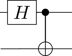
This gate sequence is of fundamental significance to quantum computing because it creates a maximally entangled 2-qubit state: a Bell state.

Playing with Q#

Having all this in mind, it is now time to have a little fun and experiment quantum programming.

Q# is a programming language used for expressing quantum algorithms. It was initially released to the public by Microsoft as part of its Quantum Development Kit.

This kit is composed of several components, the main parts being:

• Q# language and compiler: Q# is a domain-specific programming language used for expressing quantum algorithms. It is used for writing sub-programs that execute on an adjunct quantum processor under the control of a classical host program and computer.
• Q# standard library: The library contains operations and functions that support both the classical language control requirement and the Q# quantum algorithms.
• Local quantum machine simulator: A full state vector simulator optimized for accurate vector simulation and speed.

The quantum simulator that is shipped with the Quantum Development Kit is capable of processing up to 32 qubits (and up to 40 qubits on Azure).

It runs on Windows boxes, as well as on real operating systems such as GNU/Linux or MacOS.

A typical program is twofold:

• A “classical” part (using a traditional .Net programming language) is used to invoke the quantum simulator, provide input data and read output data from it
• A “quantum” part (using the Q# programming language) with the ability to create and use qubits for algorithms

The most prominent features of Q# are the ability to entangle and introduce superpositioning to qubits via CNOT and Hadamard gates.

The primitive operations are defined in the Q# standard library, like:

• Common 1-qubit unitary operations: Pauli gates (X, Y, Z), 1-qubit Cliffords like the Hadamard gate (H), …
• Phase shift gates like the T operation or Rx, Ry, Rz, … rotations
• Multi-qubits operations like CNOT, CCNOT, SWAP, …
• Measurements on single qubits like the M operation (which measures Pauli-Z operations on a single qubits) or the Mesure operation (which performs a joint measurement of one or more qubits in the specified product of Pauli operators)
• Classical functions: built-in data types (Int, Double, Range …), the Random operation, …
• Usual math operations, type conversions and bitwise operations

It sounds good to build our little playground ! But be aware that (up to now), only the libraries and samples have been open sourced (MIT license) …

Note: the following example comes almost straight out of the Q# tutorial, since it suits nicely our pedagogical purposes.

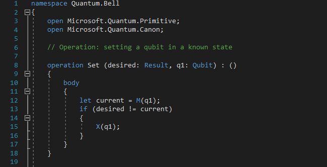
Let’s define our first operation:

• measuring a qubit (M operation)
• if it’s in the state we want, we leave it alone, otherwise, we flip it with the Pauli-X gate (X operation):

Rather straightforward ! Now, let’s introduce a second operation (Bell Test):

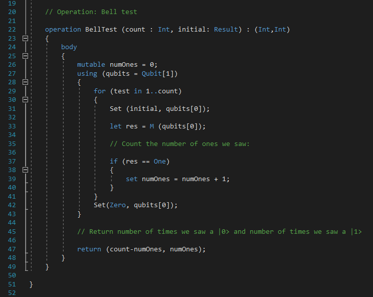
This operation loops for count iterations, sets a specified initial value on a qubit and them measures the result. It gathers statistics on how many zeros and ones are measured and returns them to the caller (“classical” part of the application). It also resets the qubit to a known state (Zero) before returning it, allowing others to allocate this qubit in a known state (required by the “using” statement, used to allocate an array of qubits for use in a block of code).

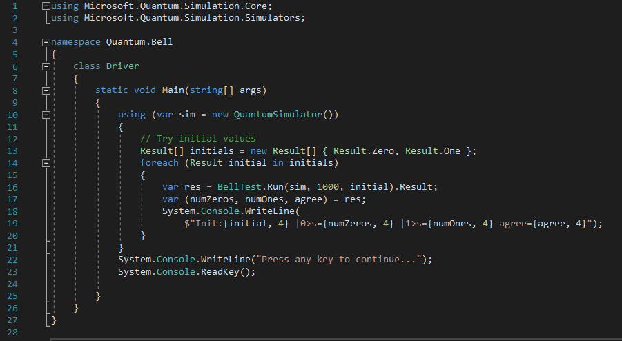
Now comes the non-quantum part :

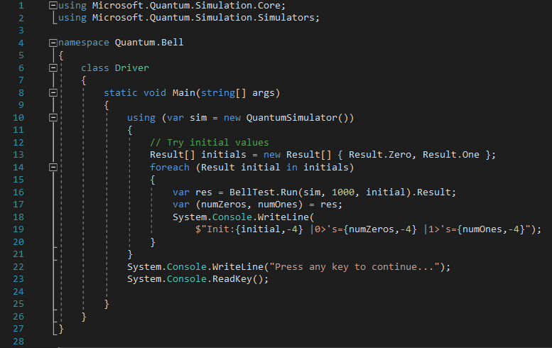
Simple enough, it:

• spawns a new Quantum simulator
• sets the input parameters needed for the quantum algorithm
• runs 1 000 times (asynchronously) for each initial values (0 and 1) the quantum algorithm and fetches the results : a tuple of the number of zeros (numZeros) and number of ones (numOnes) measured by the simulator
• Outputs the resulting statistics

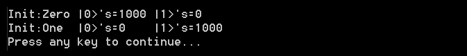
The results, unsurprisingly (since initial states are prepared to be either or ), are :

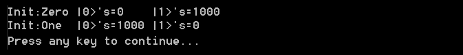
Of course, if one flips the qubits with a X gate before we measure it (in the BellTest operation):

And the results are thus reversed:

So far, these are “only” classical results. Let’s add a bit of quantum weirdness !

All we have to do is replace the X gate by an Hadamard H gate : instead of flipping the qubit all the way from to , we will only flip it halfway:

And the results are:

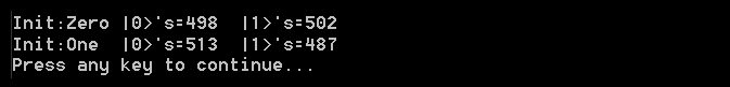
Every time a measure is performed, the qubit is halfway between and ), so one gets (statistically) 0 half the time and 1 half the time.

We have created a superposition. This gives us our first real view into a quantum state with Q# !

And now, let’s get into quantum entanglement !

For this :

• we will have to allocate 2 qubits instead of one in the BellTest operation
• this will allow us to add a CNOT gate before measurement
• we will have to add another Set operation to initialize the second qubit (to make sure it’s always in the state when we start)
• we also need to reset the second qubit before releasing it
• we’re really interested in is how the second qubit reacts to the first being measured, so we’ll have to add this statistic to the BellTest operation

The modified BellTest operation now looks like:

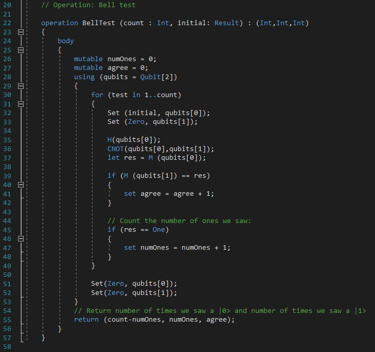
We introduced a new return value (named “agree”) that will keep track of every time the measurement from the first qubit matches the measurement of the second qubit.

Of course, we will also have to update the classical part accordingly:

And … results are:

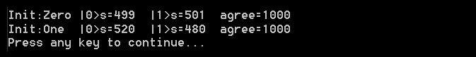
Our statistics for the first qubit haven’t changed (50-50 chance of a or a ).

But now when we measure the second qubit, it is always the same as what we measured for the first qubit. Our CNOT gate has entangled the two qubits, so that whatever happens to one of them, happens to the other !

Please note that if you reversed the measurements (the second qubit before the first), the same thing would also happen.

And there we go, these were our first steps with quantum computing using Q# 🙂

Note: to speedup the writing of this post, a few paragraphs and illustrations are based on wikipedia’s entries on quantum computing. Q# examples are based on MS Quantum Development Kit documentations