Complexity and quantum computing

In classical computing, a bit is a single piece of information that can exist in two states (1 or 0, true or false). As we have seen before, quantum computing uses qubits (2-states quantum systems) instead. Qubits can be represented by the mean of an imaginary sphere (called a Bloch sphere):

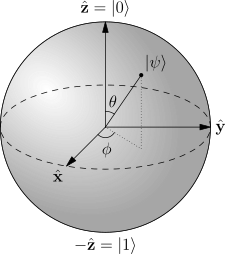
Whereas a classical bit can be in two states (pictured for example as one of two poles of the sphere), a qubit can be any point on the sphere. Points on the surface of the sphere correspond to pure states of the system, whereas the interior points would correspond to mixed states.

Unlike classical bits, qubits can thus store much more information than just 1 or 0, because they can exist in any superposition of these values. Furthermore, one can create nontrivial correlated states of a number of qubits (known as entangled states). Entanglement is a correlation that can exist between quantum particles: two or more quantum particles can be inextricably linked, even if separated by great distances.

These properties give a strong edge to quantum computing as compared to classical computing.

The “killer app” for quantum computers will most likely be simulating quantum physics. In July 2016, Google engineers used a quantum device to simulate a hydrogen molecule for the first time. Since then, IBM has managed to model the behavior of even more complex molecules. Eventually, researchers hope they’ll be able to use quantum simulations to design entirely new molecules for use in medicine for example.

But quantum computers operate on completely different principles to classical one, which also makes them really well suited to solving particular mathematical problems. Multiplying two large numbers is easy for any classical computer. But calculating the factors of a very large (say, 500-digit) number, on the other hand, is considered to be practically impossible. This strong asymmetry (multiplying is easy, factoring is hard) is widely used in the context of cryptography.

In the early 1990’s mathematicians and physicists showed that solving particular classes of mathematical problems would be dramatically sped-up by quantum computers (or even could only by solved by quantum computers). The Deutsch-Jozsa algorithm, Grover’s algorithm and Shor’s algorithm for finding the prime factors of numbers are typical examples of this quantum speedup.

Conversely there are classes of problems where quantum computers don’t have a particular edge.

But before going any further, one has to define what is complexity, what is a hard problem and what classes of problems exist. We will then be able to precise where quantum computing best fits in.

Computational complexity theory is a branch of the theory of computation focused on the classification of problems according to their inherent difficulty, and relating those classes to each other.

A computational problem is a task that can be solved by a computer, which is equivalent to stating that the problem may be solved by an algorithm.

The theory formalizes this intuition, by introducing mathematical models of computation to study these problems and quantifying the amount of resources needed to solve them.

Be careful to differentiate between:

Performance: how much time, storage or other resource is actually used when a program is run. Note that performance depends on the algorithm (code), but also on the machine, compiler, etc.
Complexity: how do the resource requirements scale : what happens as the size of the problem being solved gets larger ?

Complexity affects performance … but not the other way around ! A problem is regarded as inherently difficult if its solution requires significant resources, whatever the algorithm used.

To measure the difficulty of solving a computational problem, one may wish to see how much time the best algorithm requires to solve the problem. However, the running time may, in general, depend on the instance. In particular, larger instances will require more time to solve. Thus the time required to solve a problem (or the space required) is calculated as a function of the size of the instance (say, the size of the input in bits).

Complexity theory is interested in how algorithms scale with an increase in the input size. For instance, in the problem of finding whether a graph is connected, how much more time does it take to solve a problem for a graph with $2\times n$ vertices compared to the time taken for a graph with only $n$ vertices?

We introduced the concept of Turing machines in a previous post on quantum computing:

A Turing machine is a mathematical model of a general computing machine: it is a theoretical device that manipulates symbols contained on a strip (on one or multiple tapes). Turing machines are not intended to be practical computing technologies: they serve as a general model of a computing machine.

They are several kinds of Turing machines (deterministic, probabilistic, non-deterministic, quantum, …). A deterministic Turing machine is the most basic Turing machine, which uses a fixed set of rules to determine its future actions.

For a precise definition of what it means to solve a problem using a given amount of time and space, computational model such as the deterministic Turing machine are used.

The time required by a deterministic Turing machine M on input x is the total number of steps the machine makes before it halts and outputs the answer (“yes” or “no”).

A Turing machine M is said to operate within time f(n), if the time required by M on each input of length n is at most f(n).

Since complexity theory is interested in classifying problems based on their difficulty, one defines sets of problems based on some criteria.

For instance, the set of problems solvable within time f(n) on a deterministic Turing machine is then denoted by DTIME(f(n)).

Analogous definitions can be made for space requirements. For example, DSPACE(f(n)) defines the set of problems solvable by a deterministic Turing machine with space f(n), and PSPACE is the set of all decision problems that can be solved by a Turing machine using a polynomial amount of space.

Big-O notation

The complexity of an algorithm is often expressed using big-O notation. It is a mathematical notation that describes the limiting behaviour of a function when the argument tends towards a particular value or infinity. It is part of a family of notations collectively named Bachmann–Landau notations or asymptotic notations.

In computer science, big-O notation is used to classify algorithms according to how their running time or space requirements grow as the input size grow.

The time required by a algorithm is proportional to the number of “basic operations” that it performs. Some algorithm perform the same number of operations every time they are called.

For example, computer languages often have a size() method, which returns the size of a collection of items. The number of operations is independent of the size of the collection. We then say that methods like this (that always perform a fixed number of basic operations) require constant time.

Other methods may perform different numbers of operations, depending on the value of a parameter. Let’s imagine a class called List, and its method remove(), which has to move over all of the items that were to the right of the item that was removed (to fill in the gap). The number of moves depends both on the position of the removed item and the number of items in the list. We call the important factors (the parameters whose values affect the number of operations performed) the problem (or input) size.

Furthermore, we are usually interested in the worst case: what is the most operations that might be performed for a given problem size.

For example, as discussed above, the remove() method has to move all of the items that come after the removed item one place to the left in the array. In the worst case, all of the items in the array must be moved. Therefore, in the worst case, the time for remove() is proportional to the number of items in the list, and we say that the worst-case time for remove is linear in the number of items in the list. For a linear-time method, if the problem size doubles, the number of operations also doubles.

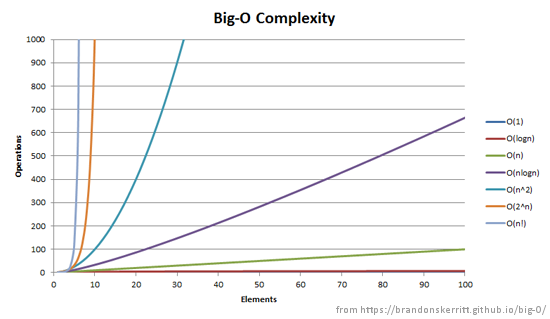
Big-O notation characterizes functions according to their growth rates: different functions with the same growth rate may be represented using the same O notation. The letter O is used because the growth rate of a function is also referred to as the order of the function. A description of a function in terms of big O notation usually only provides an upper bound on the growth rate of the function.

Let’s explore a few classical Big-O notations

$O(1)$	$O(\log n)$	$O(n),O(n^2),O(n^3),\cdots$	$O(2^n), O(2^{n^2}),\cdots$
Constant	Logarithmic	Linear, quadratic, polynomial	Exponential

As we already seen, an algorithm is said to be constant time (also written as $O(1)$ time) if the value of the running time $T(n)$ is bounded by a value that does not depend on the size of the input.

An algorithm is said to take logarithmic time if $T(n) = O(\log n)$ . Such algorithms are considered highly efficient, as the ratio of the number of operations to the size of the input decreases and tends to zero when $n$ increases. Algorithms taking logarithmic time are commonly found in operations on binary trees.

An algorithm is said to take linear time if $T(n) = O(n)$ . This means that the running time increases at most linearly with the size of the input : that there is a constant $c$ such that the running time is at most $c \times n$ for every input of size $n$ . For example, a procedure that adds up all elements of a list requires time proportional to the length of the list, if the adding time is constant, or, at least, bounded by a constant.

An algorithm is said to be of polynomial time if its running time is upper bounded by a polynomial expression in the size of the input for the algorithm, i.e., $T(n) = O(n^k)$ for some constant $k$ . All the basic arithmetic operations (addition, subtraction, multiplication, division, and comparison) can be done in polynomial time.

Finally, an algorithm is said to take superpolynomial time if $T(n)$ is not bounded above by any polynomial. For example, an algorithm that runs for $2^n$ steps on an input of size $n$ requires superpolynomial time $O(2^n)$ . Here, more specifically, it is of exponential time, which is the slowest of them all:

It is easy to understand that there are of course many other time complexities and their associated Big-O notation: $O(n!), O(n\log n), O(\sqrt{n})$ …

Complexity classes

The concept of polynomial time leads to several complexity class, some of theme defined using polynomial time :

P: The complexity class of decision problems that can be solved on a deterministic Turing machine in polynomial time.
NP: The complexity class of decision problems that can be solved on a non-deterministic Turing machine in polynomial time.
BQP: The complexity class of decision problems that can be solved with 2-sided error on a quantum Turing machine in polynomial time.

This is, of course, only a very small subset of complexity classes.

Within the NP class, there are problems that are thought to be particularly difficult. These are called NP-complete.

As an example, if you are given a map with thousands of islands and bridges, it may take years to find a tour that visits each island once. Yet if someone shows you a tour, it is easy to check whether that person has succeeded in solving the problem. This a formulation of the famous travelling salesman problem. These are problems for which a solution, once found, can be recognized as correct in polynomial time, even though the solution itself might be hard to find.

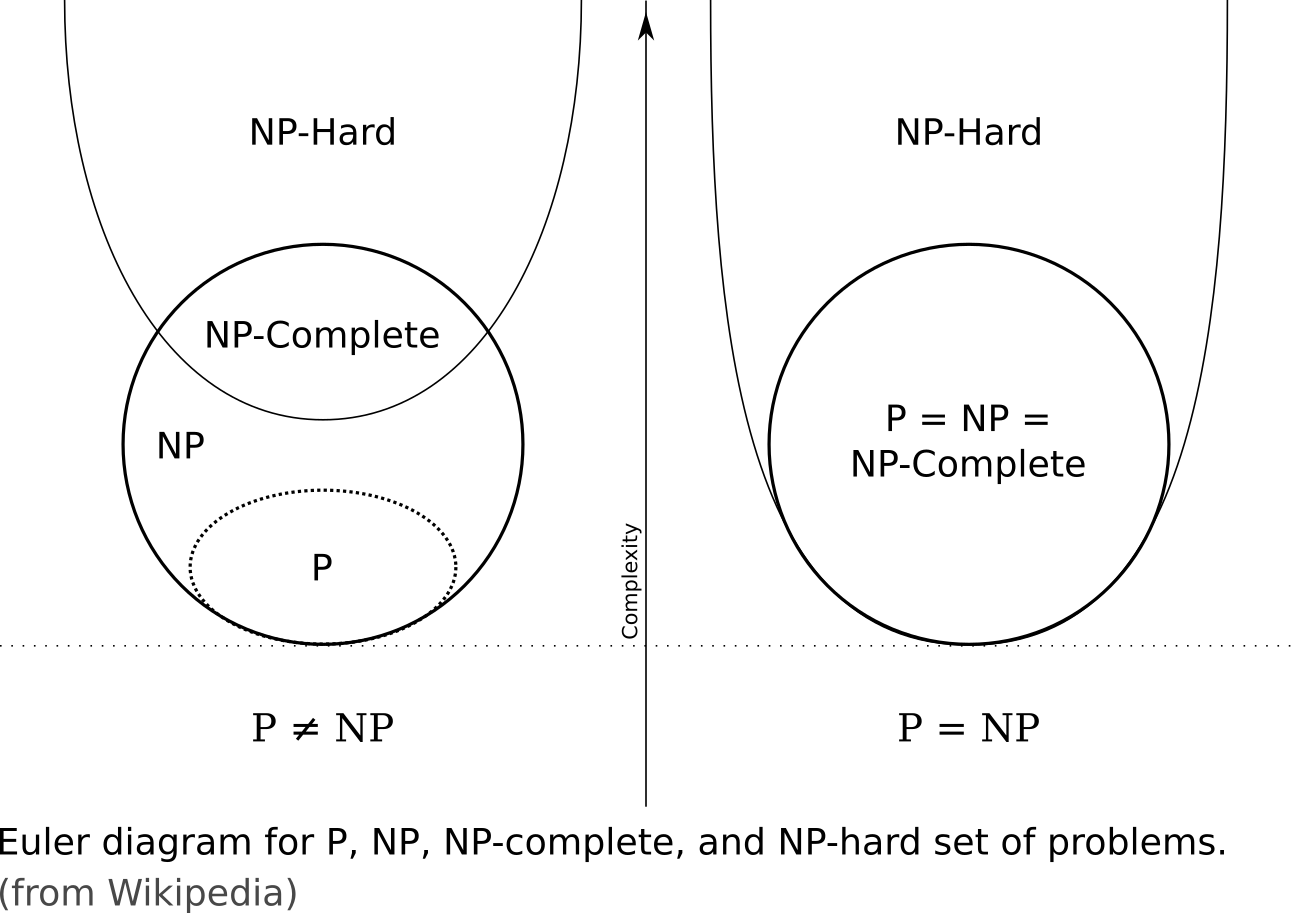
In computational complexity theory, an NP-complete decision problem is one belonging to both the NP and the NP-hard complexity classes.

Although any given solution to an NP-complete problem can be verified quickly (in polynomial time), there is no known efficient way to locate a solution in the first place; the most notable characteristic of NP-complete problems is that no fast solution to them is known. That is, the time required to solve the problem using any currently known algorithm increases very quickly as the size of the problem grows.

As a consequence, determining whether it is possible to solve these problems quickly, called the P versus NP problem, is one of the principal unsolved problems in computer science today. It is one of the seven Millennium Prize Problems selected by the Clay Mathematics Institute to carry a US$1,000,000 prize for the first correct solution.

An answer to the P = NP question would determine whether problems that can be verified in polynomial time, like Sudoku, can also be solved in polynomial time. If it turned out that P ≠ NP, it would mean that there are problems in NP that are harder to compute than to verify: they could not be solved in polynomial time, but the answer could be verified in polynomial time.

In the half a century since the problem was recognized, no one has found an efficient algorithm for an NP-complete problem. Consequently, computer scientists today almost universally believe P does not equal NP, or P ≠ NP, even if we are not yet smart enough to understand why this is or to prove it as a theorem.

“The hardest problems” of a class refer to problems which belong to the class such that every other problem of that class can be reduced to it. A problem is said to be NP-hard if an algorithm for solving it can be translated into one for solving any NP-problem. NP-hard therefore means “at least as hard as any NP-problem,” although it might, in fact, be harder:

Quantum complexity

The class of problems that can be efficiently solved by quantum computers is called BQP, for “bounded error, quantum, polynomial time”.

Quantum computers only run probabilistic algorithms, so BQP on quantum computers is the counterpart of BPP (“bounded error, probabilistic, polynomial time”) on classical computers.

It is defined as the set of problems solvable with a polynomial-time algorithm, whose probability of error is bounded away from one half. A quantum computer is said to solve a problem if, for every instance, its answer will be right with high probability. If that solution runs in polynomial time, then that problem is in BQP.

BQP is not the only quantum complexity class. QMA, which stands for “Quantum Merlin Arthur”, is the quantum analog of the non-probabilistic complexity class NP or the probabilistic complexity class MA. It is related to BQP in the same way NP is related to P, or MA is related to BPP.

QIP, which stands for “Quantum Interactive Polynomial time”, is another complexity class. It is the quantum computing analogue of the classical complexity class IP, which is the set of problems solvable by an interactive proof system with a polynomial-time verifier and one computationally unbounded prover.

Since QMA and QIP are related to interactive proof systems, for the sake of simplicity, we are going to skip these two quantum complexity classes. Furthermore, based on a series of recent results, it is believed that QIP = PSPACE.

One of the main aims of quantum complexity theory is to find out where these classes lie with respect to classical complexity classes such as P, NP, PSPACE and other complexity classes.

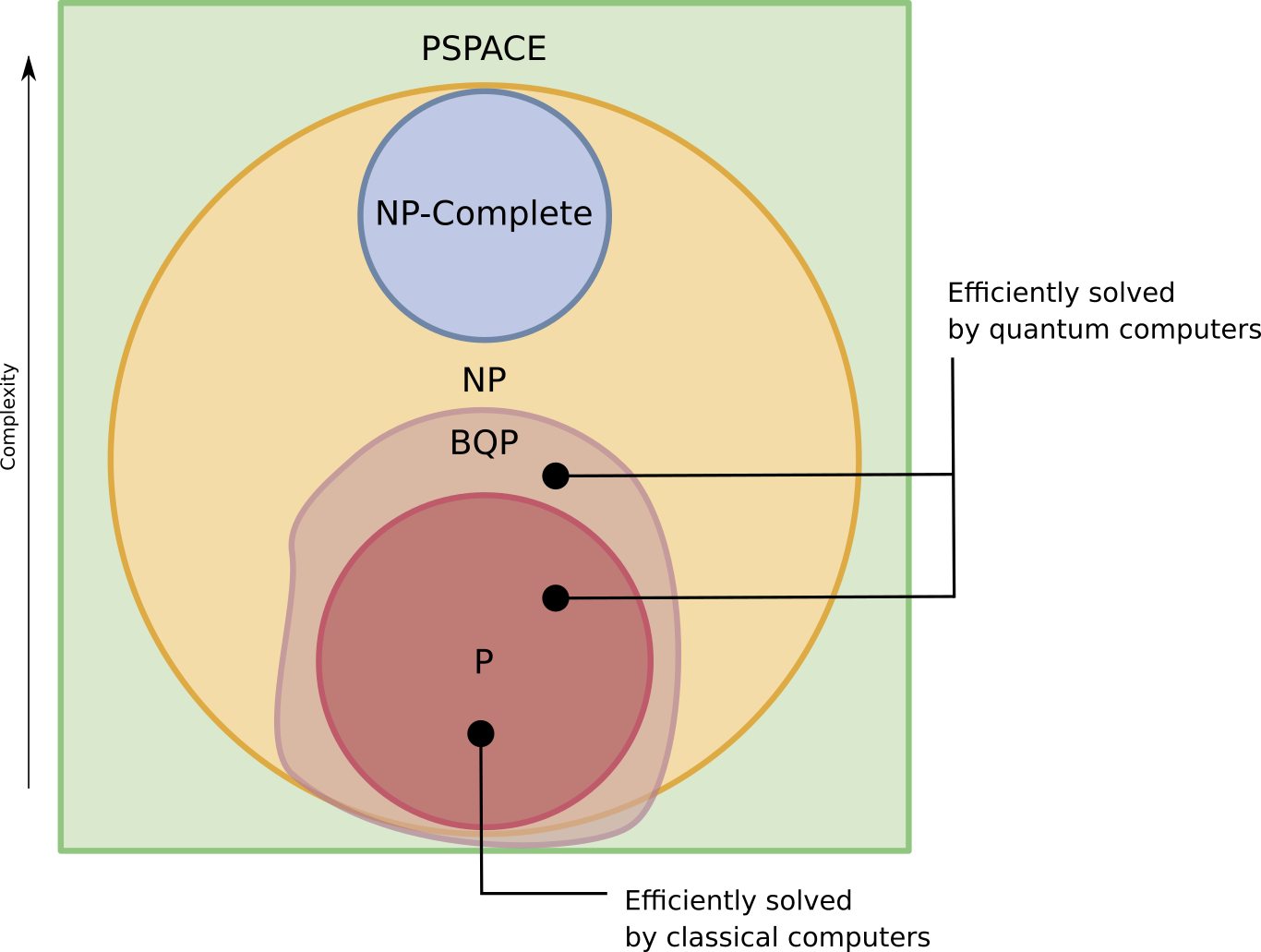
The current hypothesis is that NP-Complete and BQP are disjoint sets. Which means that any problem that is NP-Hard would still be hard for a quantum computer, although there are more efficient solutions in Quantum computers, all they give is a polynomial improvement in a exponential solution, which means final complexity is still exponential.

The BQP class includes all the P problems and also a few other NP problems (such as factoring and the discrete logarithm). Most other NP and all NP-complete problems are believed to be outside BQP, meaning that even a quantum computer would require more than a polynomial number of steps to solve them.

In addition, BQP might protrude beyond NP, meaning that quantum computers could solve certain problems
faster than classical computers could even check the answer. To date, however, no convincing example of such a problem is known. Computer scientists do know that BQP cannot extend outside PSPACE, which also contains all the NP problems:

Of course, any problem that is impossible for a normal computer (an undecidable problem), is still undecidable for a quantum computer: a Turing machine can simulate these quantum computers, so such a quantum computer could never solve an undecidable problem like the halting problem.

So why does quantum computing make sense ?

It does precisely because BQP includes a set of NP problems : there is set of problems that have not been able to prove to be NP-Complete, but for which we have no polynomial time solution yet, like Integer Factorization or Discrete Log, all of which can be solved easily by a quantum computer.

Conversely, there are problems which are out of BQP’s reach. It means, among other things, that it is possible (though quite complicated) to build quantum-resistant cryptography.

Quantum speedups

The following algorithms provide speedups over the best known classical algorithms:

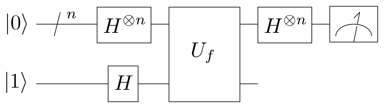
Deutsch–Jozsa’s algorithm: as we have seen in a previous post, the Deutsch–Jozsa algorithm is specifically designed to be easy for a quantum algorithm and hard for any classical algorithm. The motivation is to show a black box problem that can be solved efficiently by a quantum computer with no error, whereas a deterministic classical computer would need exponentially many queries to the black box to solve the problem:

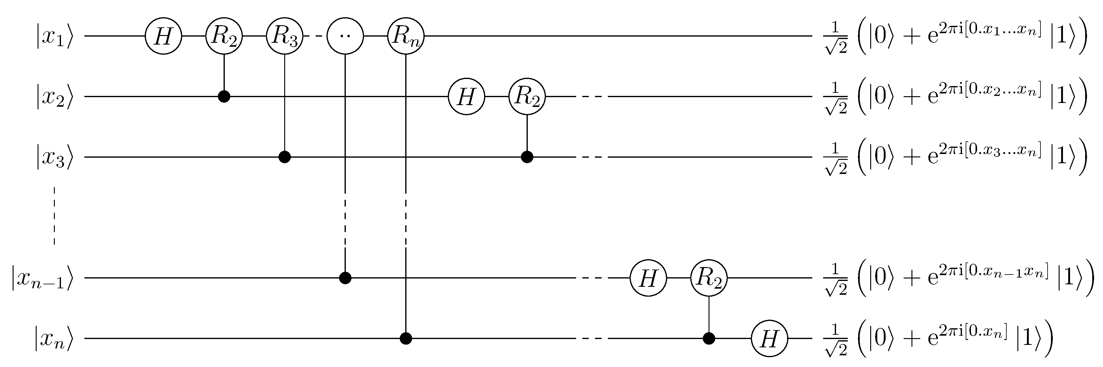
Quantum Fourier transform (QFT): the quantum Fourier transform is a linear transformation is the quantum analogue of the discrete Fourier transform. QFT is a part of many quantum algorithms, notably Shor’s algorithm for factoring and computing the discrete logarithm, or the quantum phase estimation algorithm for estimating the eigenvalues of a unitary operator. The best QFT algorithms known require only $O(log n)$ , compared with the classical discrete Fourier transform, which takes $O(n2^n)$ :

Shor’s algorithm: QFT is used in Shor’s algorithm (as seen in the following quantum circuit). This algorithm finds the prime factorization of an n-bit integer in $O(n^3)$ time whereas the best known classical algorithm requires $2^{O(n^{1/3})}$ time.

This algorithm is important both practically and historically for quantum computing. It was the first polynomial-time quantum algorithm proposed for a problem that is believed to be hard for classical computers (superpolynomial quantum speedup). This hardness belief is so strong that the security of today’s most common encryption protocol, RSA, is based upon it. A quantum computer successfully and repeatably running this algorithm has the potential to break this encryption system.

Grover’s algorithm: devised by Lov Grover in 1996, this quantum algorithm for searching an unsorted database with $n$ entries in just $O(\sqrt{n})$ , whereas the analogous problem in classical computation cannot be solved in fewer than $O(n)$ :

Now that we know a little bit more on quantum complexity, we are ready for posts on quantum cryptography 🙂

Note: to speedup the writing of this post, a few paragraphs and illustrations are based on wikipedia’s entries on quantum computing and on complexity theory.

Leave a Reply Cancel reply